Build the first haulage scenario

In this section, we start a new MineTwin Underground scenario and fill only the minimum data needed for the first working model. We will use the wizard to create the scenario shell, then we will draw a small manual geometry instead of importing a full mine layout.

We build the scenario incrementally, from the first stope and LHD haulage run to a complete material flow chain with truck haulage, conveyor transport, skip hoisting, and final storage. In this first training page, we keep the geometry schematic so we can focus on the required objects, connections, and scheduling behavior.

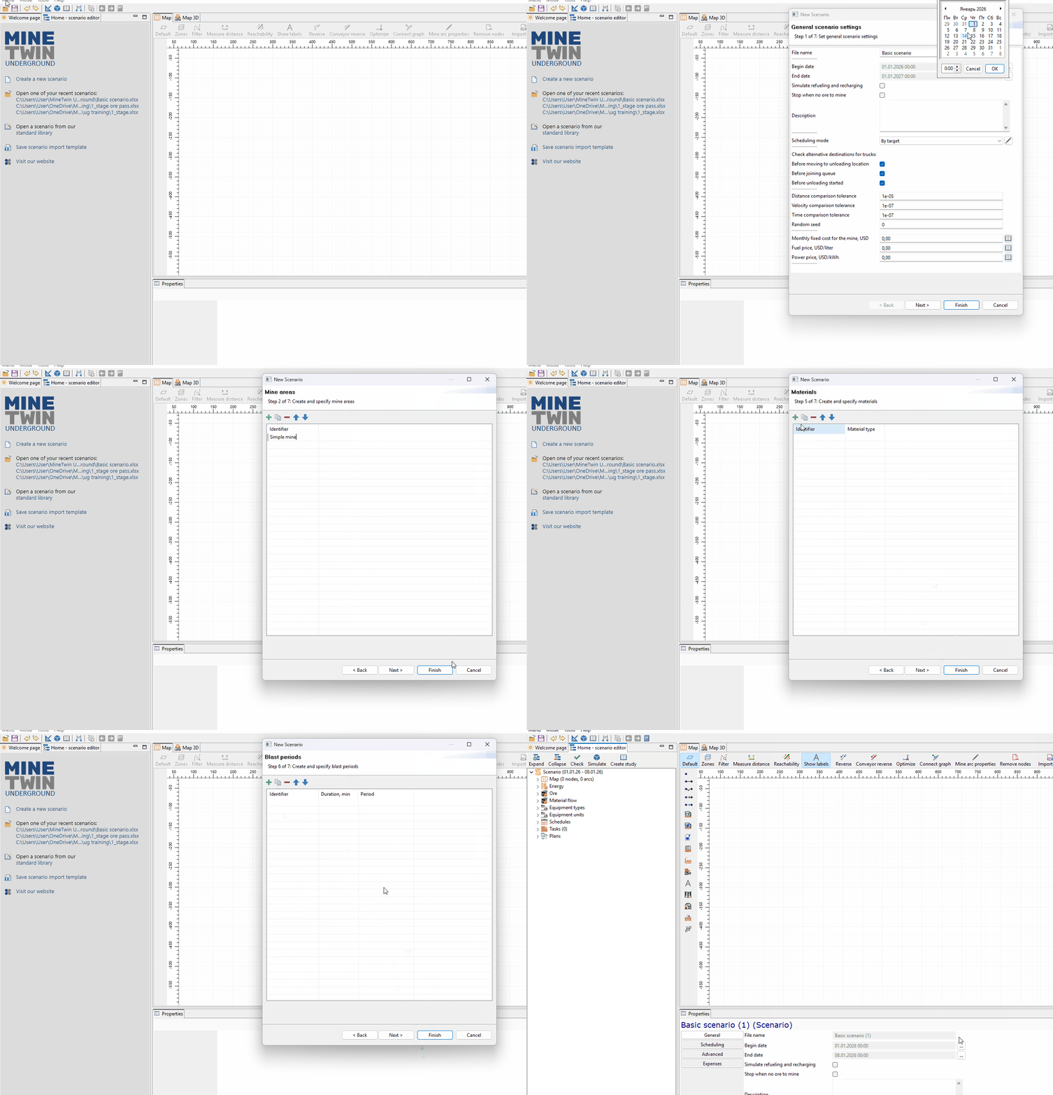
We begin from the MineTwin Underground welcome page and create a new scenario using the wizard. We click Create a new scenario, set the scenario name and planning period, and keep the wizard configuration intentionally small. We add one mine area named Simple mine, because the first model has only one operating area and does not yet need area-based equipment restrictions. We define the production ore type as Copper ore and define two materials for grade calculation: Copper as the useful substance and Rock as empty rock. We also create the basic shift pattern that will control when the LHD can work. After we finish the wizard, MineTwin opens an empty scenario editor with the Map view ready for the manual geometry that we will draw next.

Download the intermediate scenario after the wizard

In this section, we draw the first manual underground network. We will create three connected sections: the stope excavation section, the long road toward the ore pass, and a short branch to the equipment depot.

This geometry is deliberately schematic. MineTwin can still use it for routing because the roads are represented by connected mine nodes and arcs.

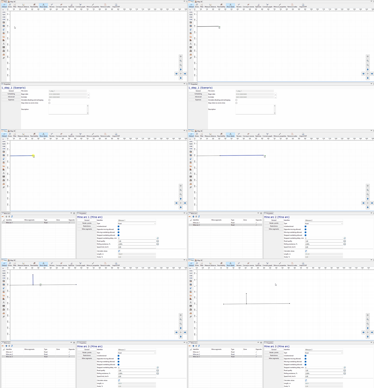
We select the mine polyline tool and draw the first section that will become the stope excavation. Then we continue the line to create the long road from the stope area toward the future ore pass. Finally, we draw a short branch from the main road to the depot point. This geometry gives us a simple route where the LHD can start near the depot, travel to the stope, and haul ore directly to the ore pass.

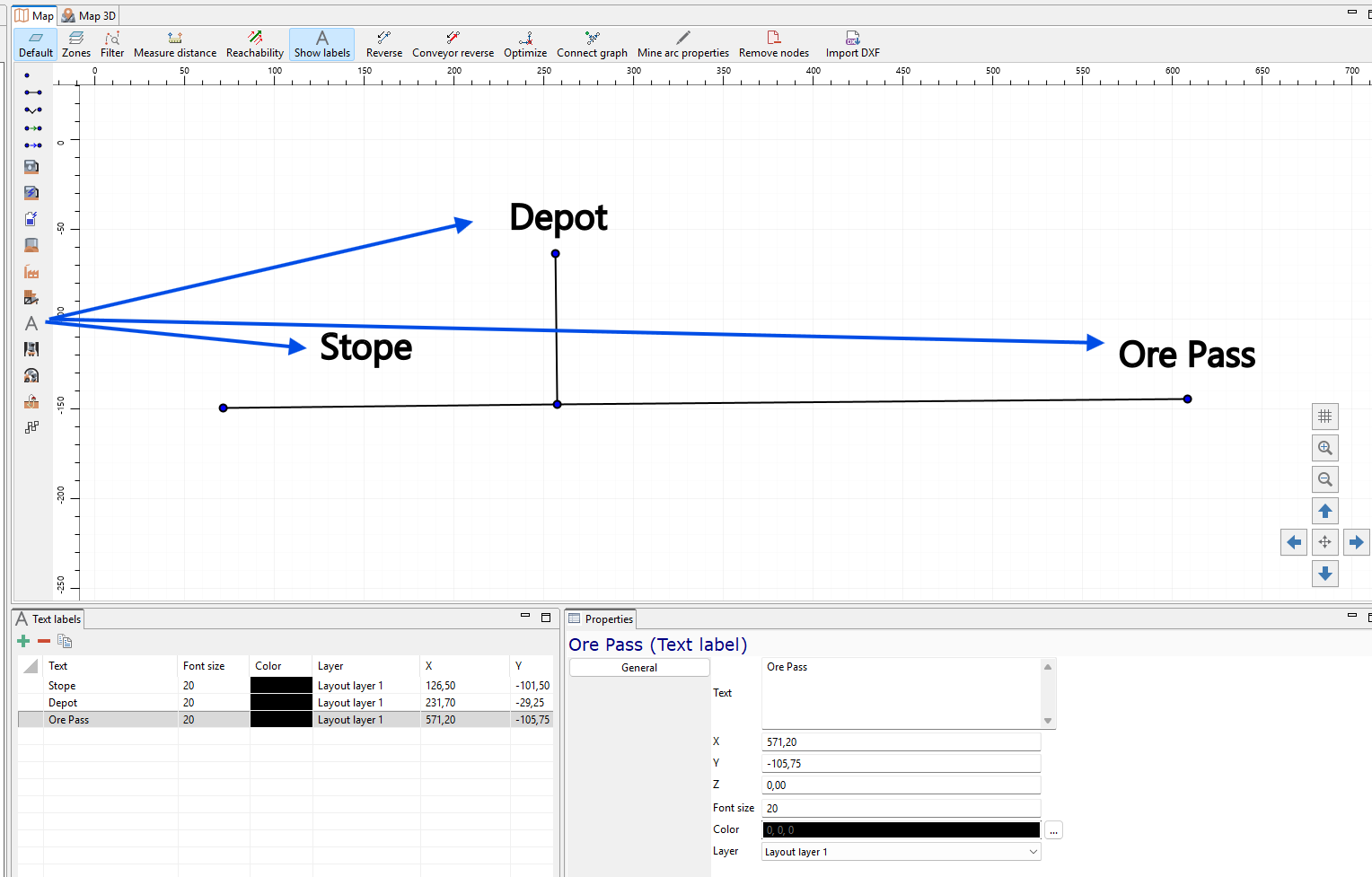
We add text labels to make the schematic geometry easy to read during the guided demonstration. The labels identify the stope, the depot point, and the future ore pass location. They do not change the simulation logic, but they make the map easier to explain while we add the scenario objects.

Download the intermediate scenario after drawing and labeling the geometry

In this section, we turn the first road section into a mineable part of the scenario. We will create a mine segment for the selected mine arc and then use that segment as the location of the stope.

Mine segments connect mine arcs with mining fronts. For this first example, we keep the relationship simple: one selected mine arc becomes one mine segment for one stope.

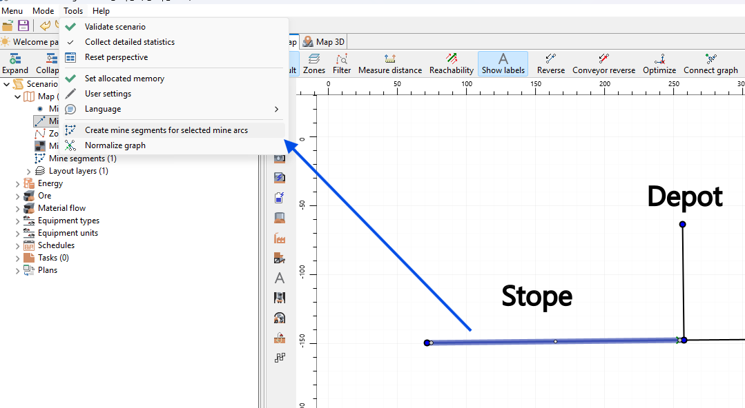
We select the mine arc under the Stope label and use the Create mine segments for selected mine arcs command from the Tools menu. MineTwin creates a mine segment on the selected arc, which gives us the network location needed for the future stope.

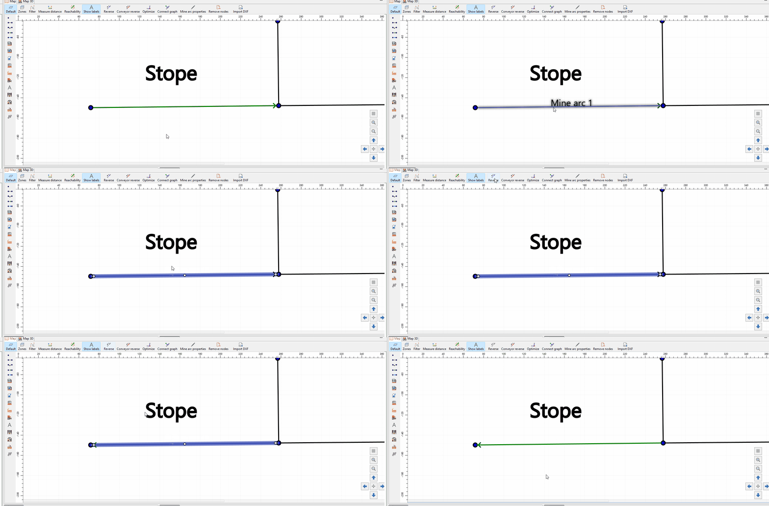
We reverse the direction of the mine segment so that the stope advances in the intended direction. The direction matters because it defines how the mining front progresses along the selected road section.

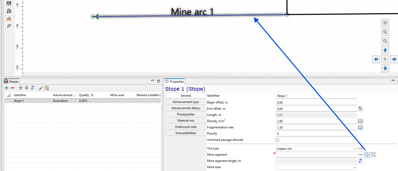
We create Stope 1 and assign the prepared mine segment to it using the crosshair button in the stope properties. This connects the stope object with the selected road section on the map, so MineTwin knows where the mining front is located.

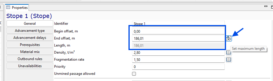
We use the Set maximum length button to make the stope occupy the whole mine segment. The begin offset remains 0 m, and the end offset is set to the full segment length shown by MineTwin.

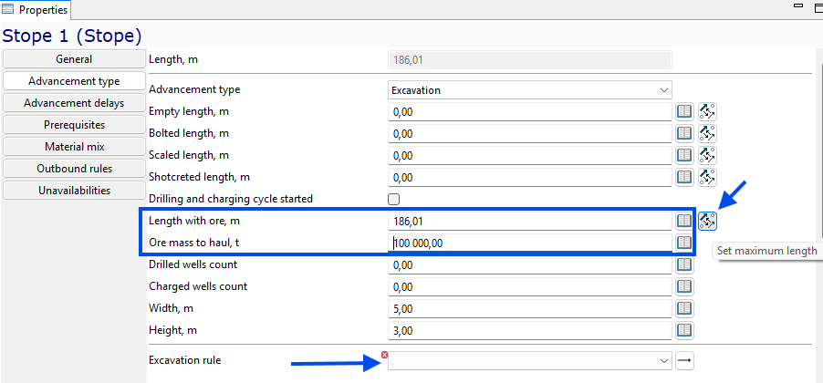
We keep the advancement type as Excavation and use the length button to fill the whole stope length with ore ready for haulage. For the first simulation, we do not model drilling, charging, or blasting yet. We set Ore mass to haul to 100,000 t so the LHD has enough material to move during the demonstration. MineTwin also shows that an Excavation rule is required because the stope advancement type is Excavation. We will create this rule next.

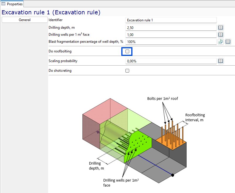
We create Excavation rule 1 and keep the default drilling-related settings for now. To keep the first scenario simple, we clear Do roofbolting. This means we do not need to add roof bolting equipment before the first LHD haulage demonstration.

We return to Stope 1 and select Excavation rule 1 from the Excavation rule dropdown in the Advancement type properties. This completes the required link between the stope’s excavation advancement type and the rule that defines the excavation settings.

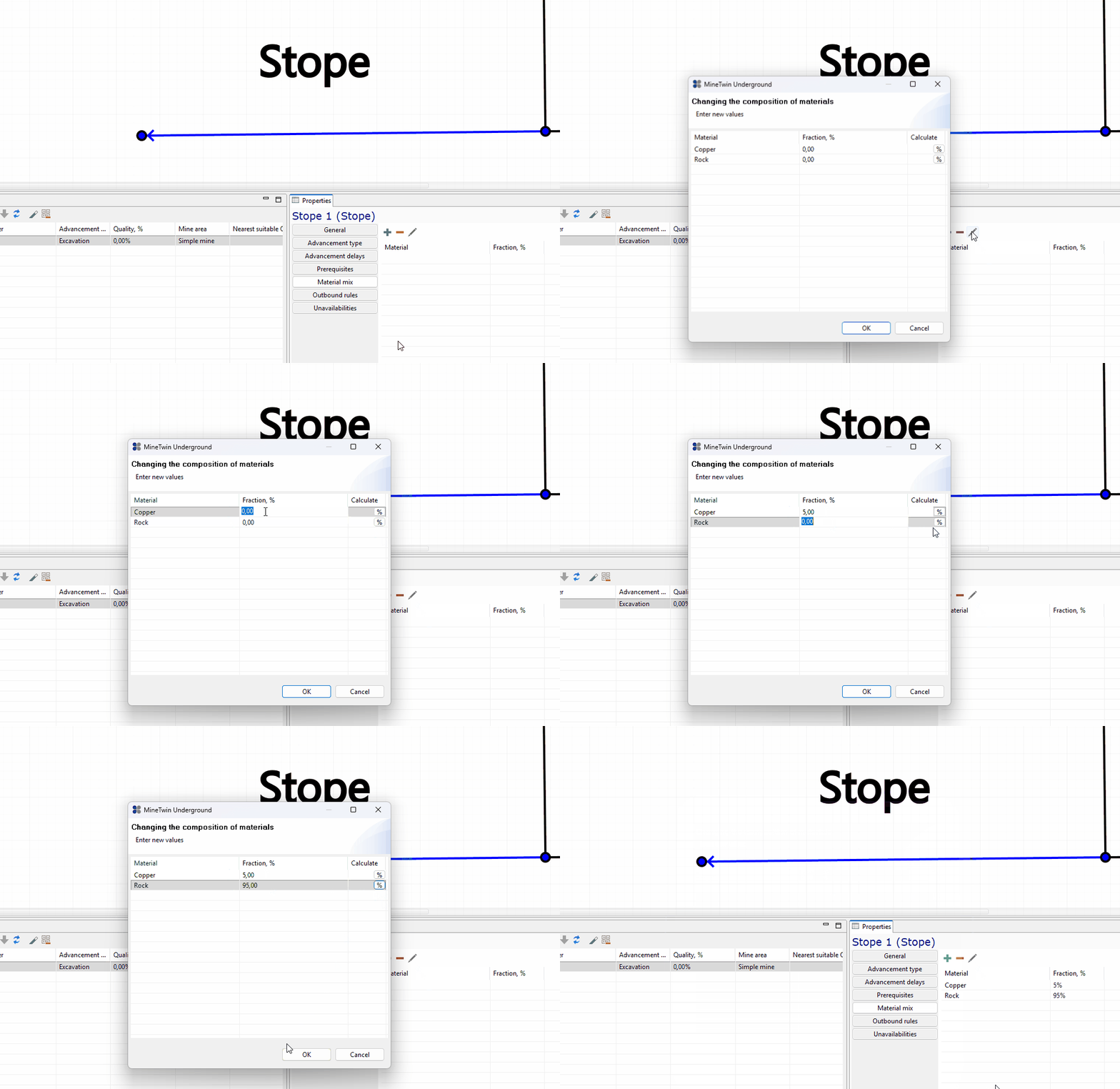
We use the material mix helper to define the ore grade for Stope 1. For this training scenario, we set the stope to 5% Copper and 95% Rock. MineTwin uses this material mix to calculate the stope quality shown in the stopes table.

Download the intermediate scenario after configuring the first stope

In this section, we add the ore pass and begin preparing the mobile equipment for the first haulage run. The ore pass will be the destination for the ore hauled from Stope 1.

MineTwin uses the ore pass connection to determine where material can be unloaded. After the ore pass and LHD are configured, MineTwin will be able to build a route from the stope to the ore pass through the road network.

We create the ore pass near the end of the long road and assign its inbound node using the map selection tool. This connects the ore pass object to the road network, so the LHD will have a valid unloading destination for the ore from the stope.

We add the LHD type from the MineTwin equipment library. For this scenario, we select Epiroc Scooptram ST14 and import it into the scenario. The library fills the main loader parameters, including capacity, volume, loading duration, unloading duration, and loaded and empty speeds.

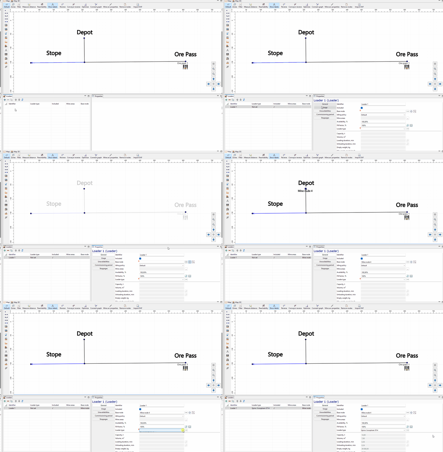
We create one loader unit for the scenario. We select the imported Epiroc Scooptram ST14 type from the loader type list and assign the unit’s base node at the depot. The base node defines the LHD’s initial position when the simulation starts.

Download the intermediate scenario after adding the ore pass and LHD

In this section, we check whether the scenario has enough information for the first simulation run. The model now has a stope, an ore pass, and one LHD, but MineTwin still needs a production target because the scenario uses target-based scheduling.

This check is useful before every first run. It tells us which required planning or simulation inputs are still missing, so we can fix them before switching to simulation mode.

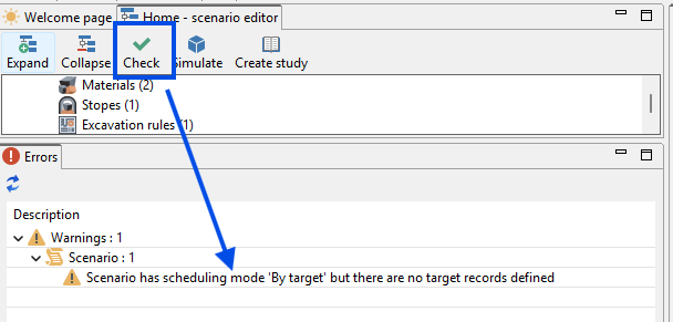
We run the scenario check and review the warning in the Errors view. MineTwin tells us that the scenario has scheduling mode By target, but no target records are defined.

We create the first target plan record. For this one-week scenario, we set mining type to Production, quality to 5%, and planned mass to 100,000 t. This target gives MineTwin the production goal that the scheduler will use in the first simulation run.

In this section, we make the first complete run of the simple underground haulage scenario. At this point, the model has the minimum connected set of objects: one stope with available ore, one ore pass, one LHD, and a production target.

We use this run as a functional check rather than a detailed performance analysis. The main goal is to confirm that MineTwin can build the route automatically and animate the first haulage cycle from the stope to the ore pass.

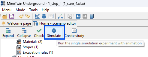
We click Simulate to start a single simulation experiment with animation. MineTwin switches from the scenario editor to the simulation view and prepares the model for playback.

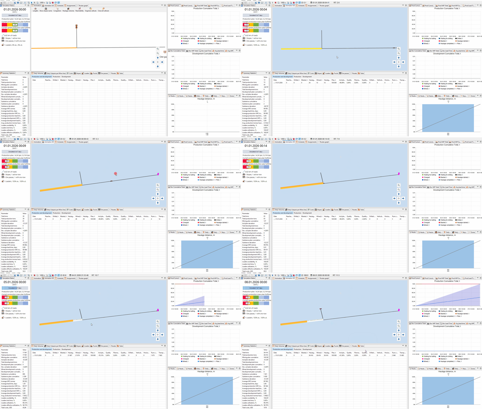
We review the animated run and watch the LHD move through the road network. The loader starts from its base node, travels to the stope, hauls ore along the long road, and unloads it into the ore pass. This confirms that the stope, ore pass, road network, loader unit, and target plan are connected correctly for the first run. On the map, we also see the yellow line in the stope become shorter as the available ore volume in the excavation decreases. In the simulation status panel, we can already compare the current production with the plan, and the first run shows that the scenario is still behind the target.

Download the intermediate scenario after the first simulation run

In this section, we start preparing the second haulage leg that will later be served by trucks. The LHD will continue to work on the first haulage leg, from the stope to the first ore pass. The truck will work on the next leg, moving material from the first ore pass toward a second ore pass.

We will build this second leg as a compact schematic geometry with realistic transport properties. First, we create a lower road section on the -50 m level. Then we label the two ore pass locations, set a custom haulage length for the second leg, and connect the two levels with a ramp.

This step prepares the geometry for the next operating pattern. The model will still have the LHD hauling from the stope to Ore Pass #1, and the truck route will be added on the geometry from Ore Pass #1 toward Ore Pass #2.

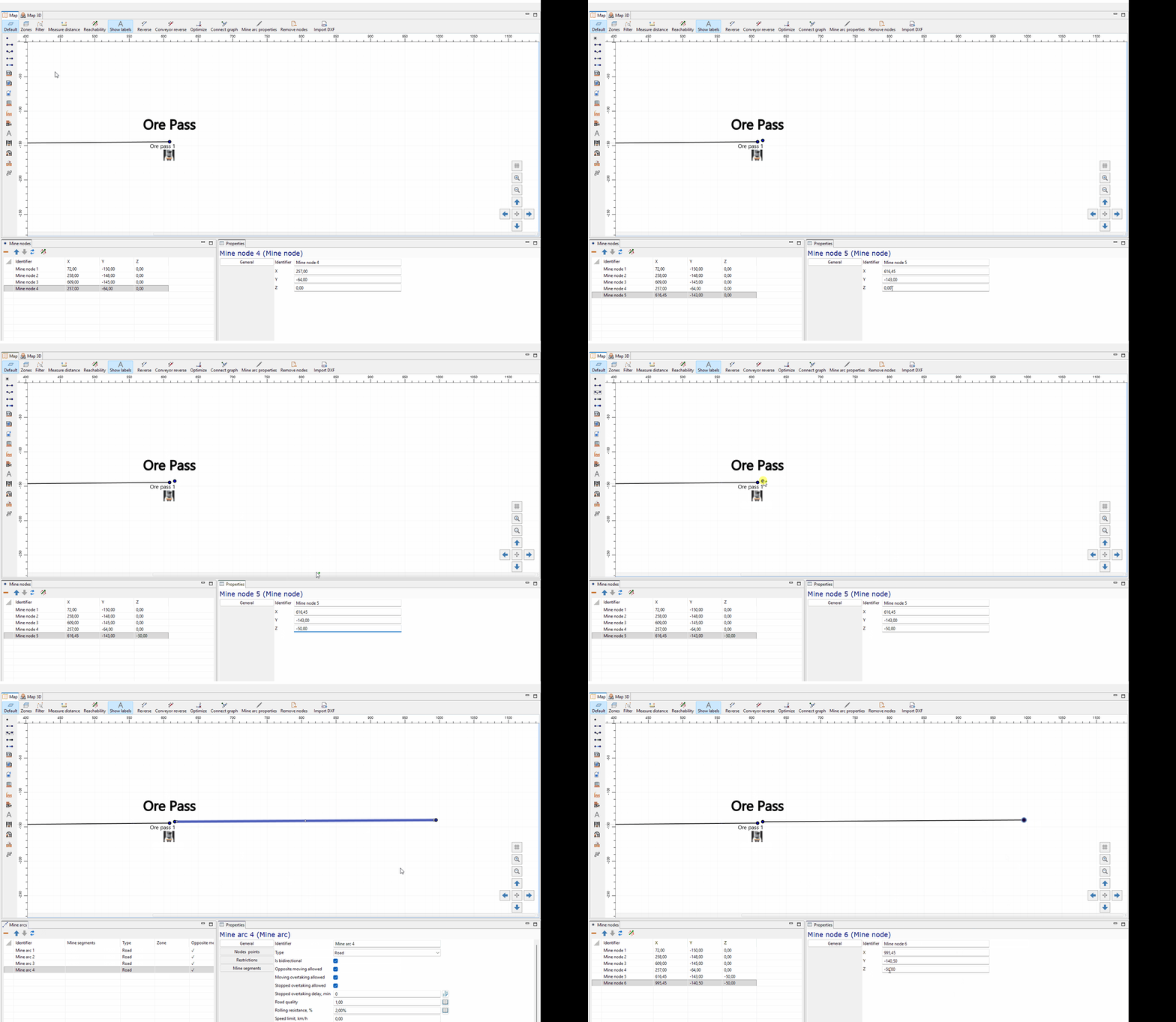
We create a new mine node away from the existing road network and set its Z coordinate to -50 m. Then we draw a mine polyline from this node to create the second haulage leg. MineTwin keeps the elevation for the next point of the polyline, so the resulting arc is created on the same -50 m level. This is important because the Z coordinate belongs to mine nodes and is used later for slope and gradient calculations on the road network.

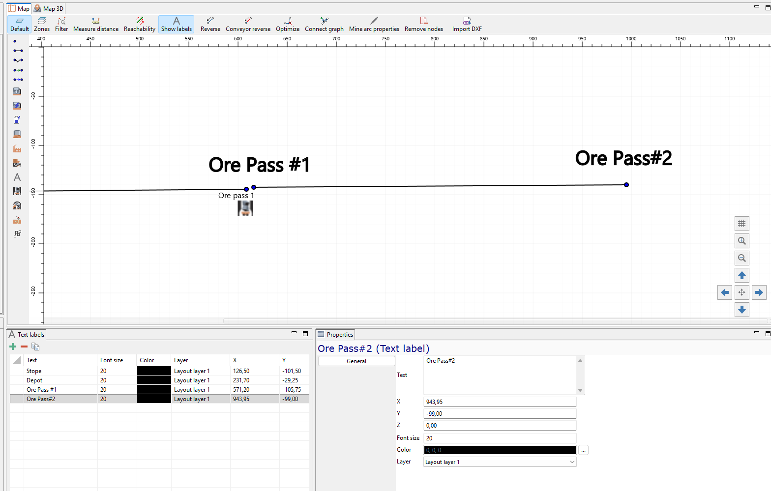
We update the existing label near the first ore pass so it reads Ore Pass #1. Then we add a new label at the far end of the second haulage leg and name it Ore Pass #2. These labels help us explain the transfer scheme on the map: the LHD delivers material to the first ore pass, and the truck will later move material from the first ore pass toward the second ore pass. The labels are only visual annotations, so we will still create and connect the actual second ore pass object separately.

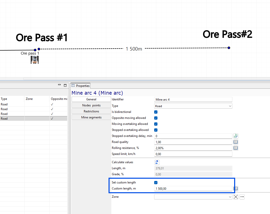
We select the new mine arc and enable Set custom length in its properties. The drawn arc is shorter on the schematic map, but we set its custom length to 1,500 m. This lets us keep the training geometry compact on screen while still modelling a realistic truck haulage distance between the first and second ore pass locations.

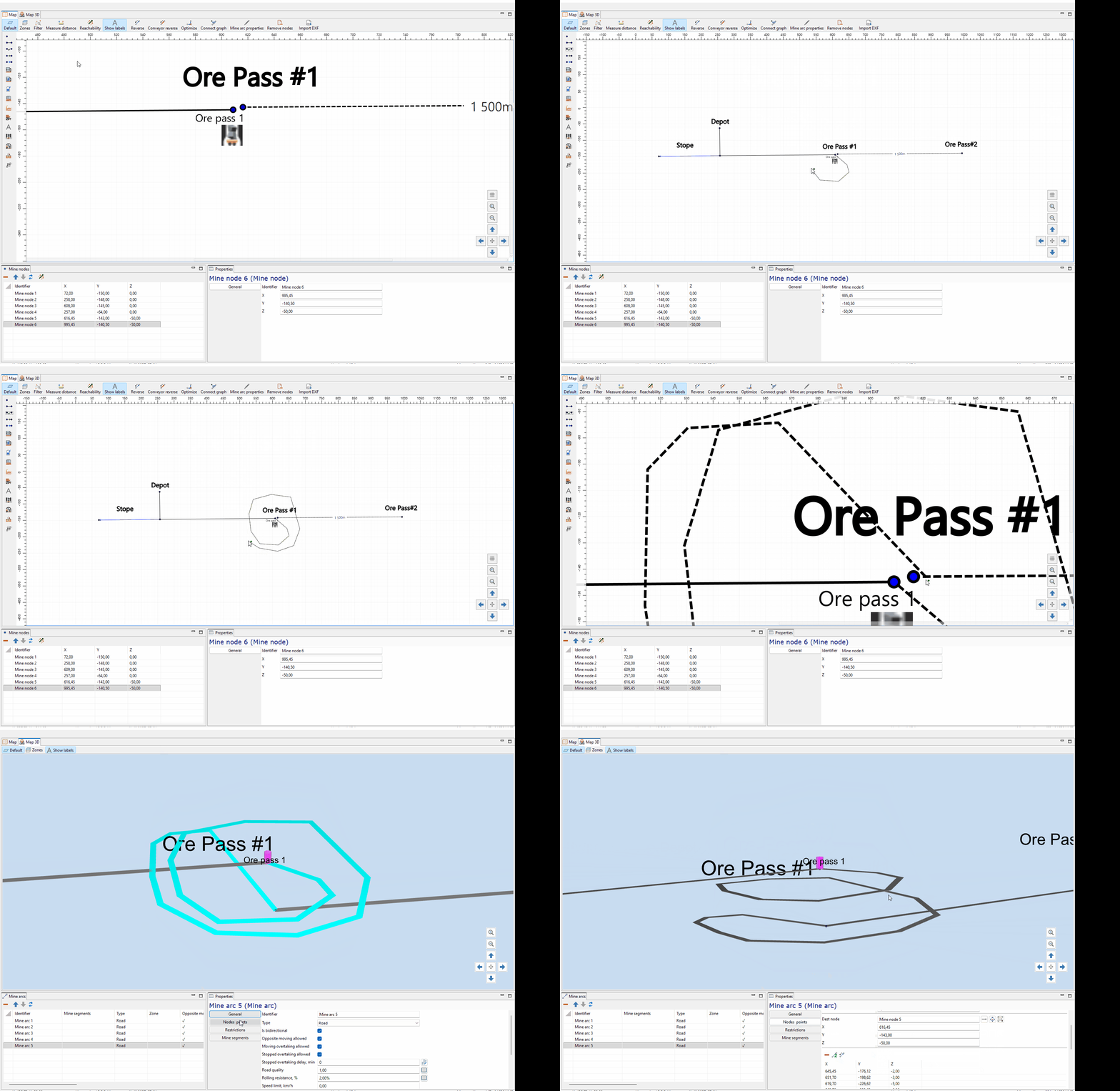
We draw a connecting polyline between the first haulage leg and the new lower haulage leg. This creates a ramp between the 0 m level and the -50 m level. After drawing the ramp, we use the special height distribution button to spread the Z coordinates evenly across the intermediate bend points. MineTwin then calculates a smooth elevation transition along the ramp, which will be used later for route gradients.

Download the intermediate scenario after creating the second haulage leg geometry

In this section, we start turning the second haulage leg into an operating transfer system. We adjust the existing ore pass, add the second ore pass, and add truck equipment for the haulage route between them.

This completes the first transfer chain in the scenario. The LHD delivers material from the stope to Ore pass 1, and the truck hauls material from Ore pass 1 to Ore pass 2.

We also check the scheduling behavior after the truck is added. This lets us see why the first run does not dispatch the truck immediately and how dynamic haulage scheduling changes that behavior.

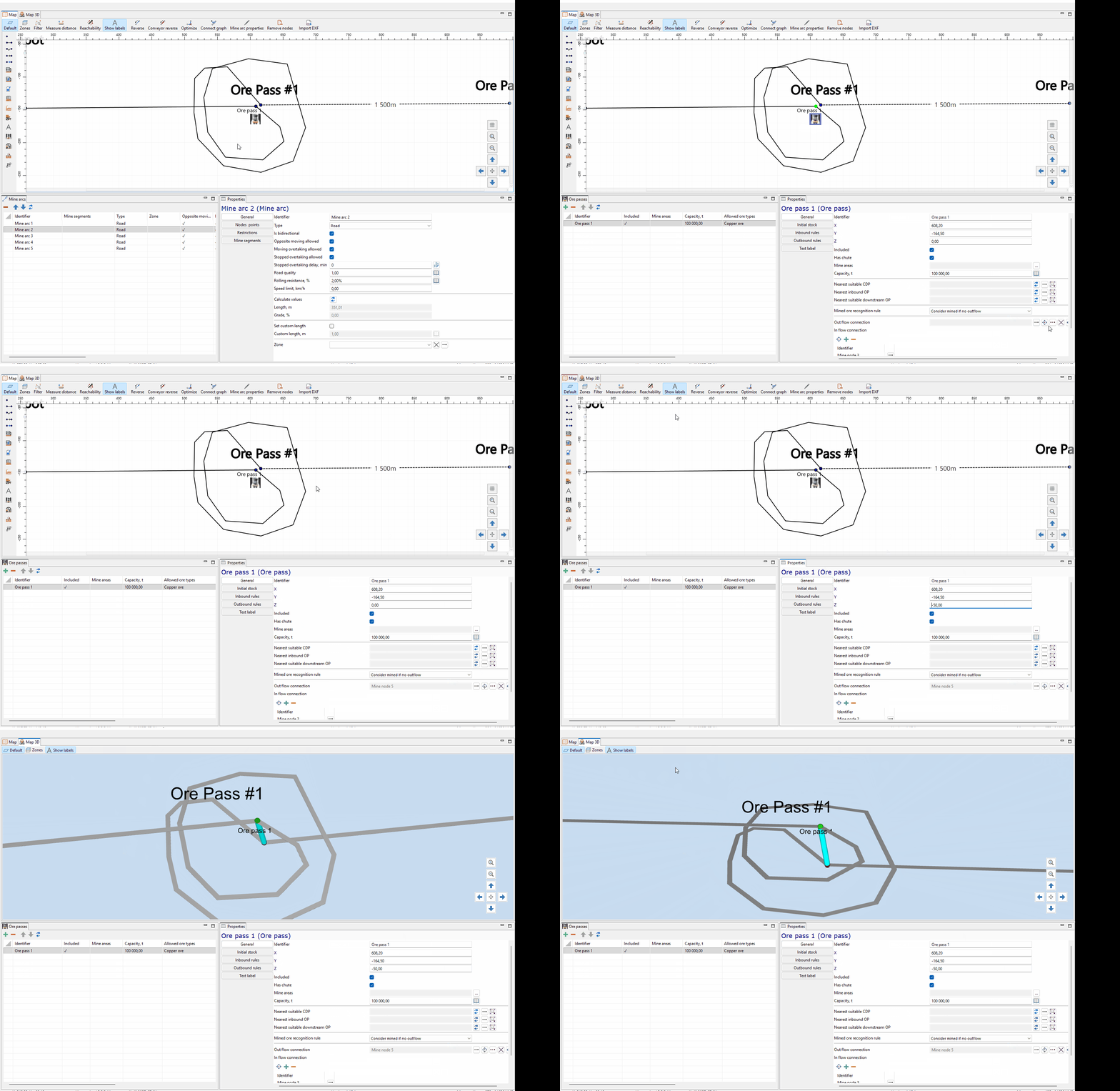
We select the existing ore pass and assign its outbound node at the start of the second haulage leg. This defines where ore leaves the ore pass and becomes available for truck loading. Because an ore pass has a chute, the truck can load under it directly, without a separate loader at this transfer point.

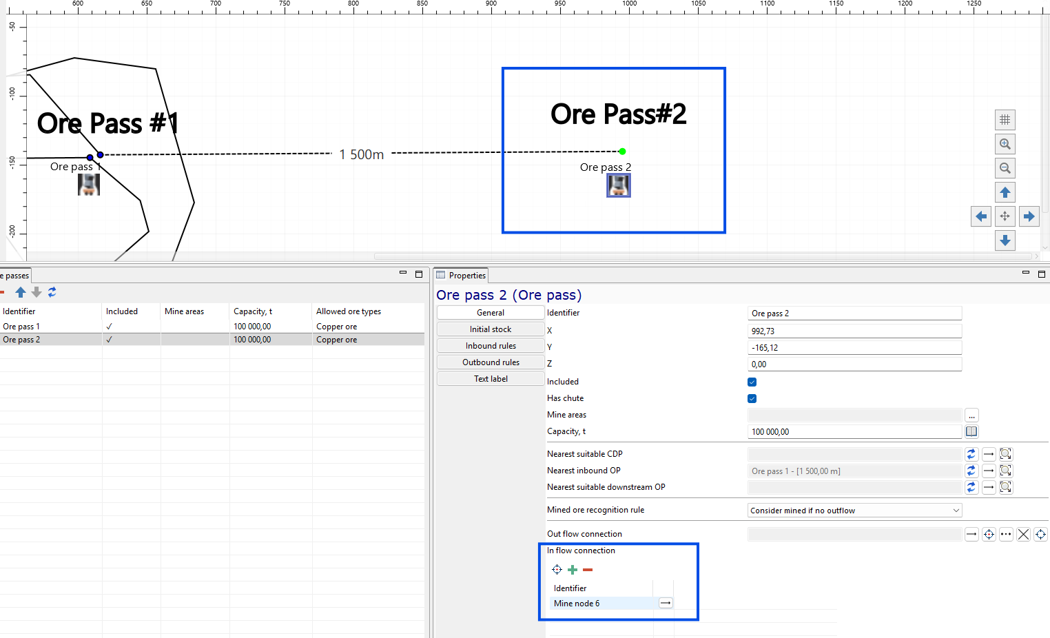
We create Ore pass 2 at the far end of the second haulage leg. We allow the same Copper ore type and keep the capacity at 100,000 t for this training scenario. Then we assign the inbound connection to the end node of the second leg, so trucks will have a valid unloading destination after hauling material from Ore pass 1. MineTwin now recognizes Ore pass 1 as the nearest inbound ore pass for Ore pass 2 through the 1,500 m haulage leg.

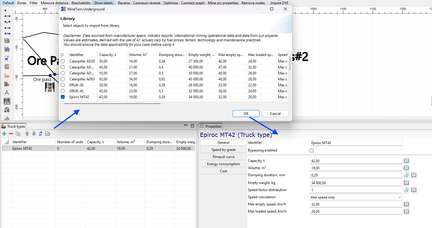
We add a truck type from the MineTwin equipment library. For this scenario, we select Epiroc MT42 and import it into the truck types table. The library fills the main truck parameters, including capacity, volume, dumping duration, and empty weight. This prepares the equipment type that we will use for the truck units on the second haulage leg.

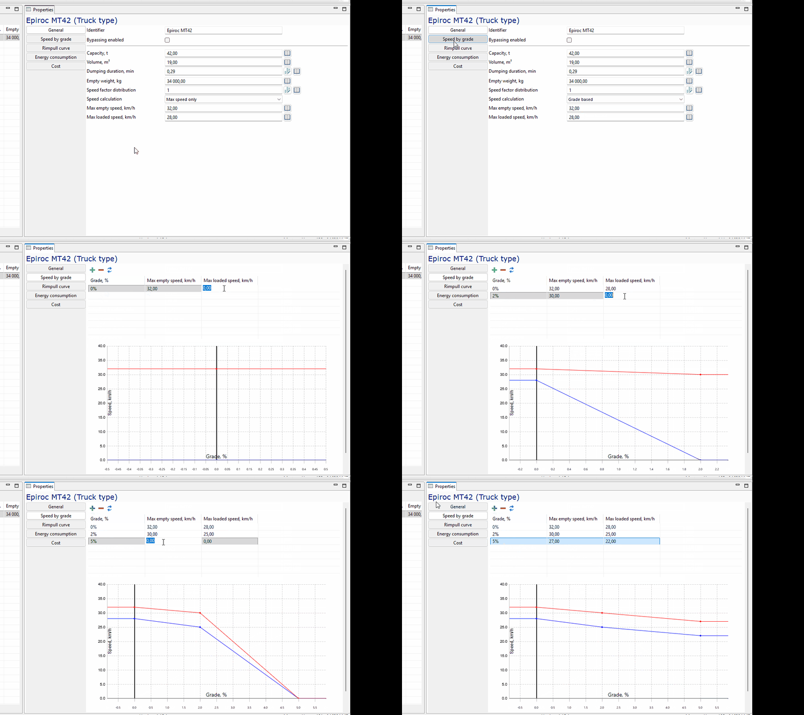
For illustration, we define truck speed by road grade instead of using only one maximum speed. We open the Speed by grade settings for Epiroc MT42 and add speed rows for 0%, 2%, and 5% grade. For empty travel, we set maximum speeds of 32 km/h, 30 km/h, and 27 km/h. For loaded travel, we set maximum speeds of 28 km/h, 25 km/h, and 22 km/h. This gives MineTwin a simple speed curve that slows the truck down as the grade increases.

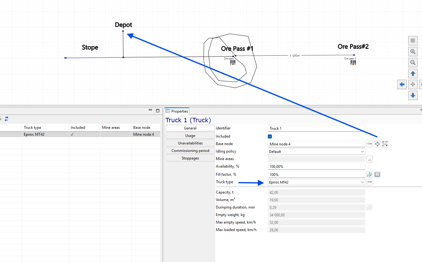
We create Truck 1 as the first truck unit in the scenario. We assign the Epiroc MT42 truck type and place the truck at the depot by selecting Mine node 4 as its base node. The base node defines the truck’s initial position when the simulation starts.

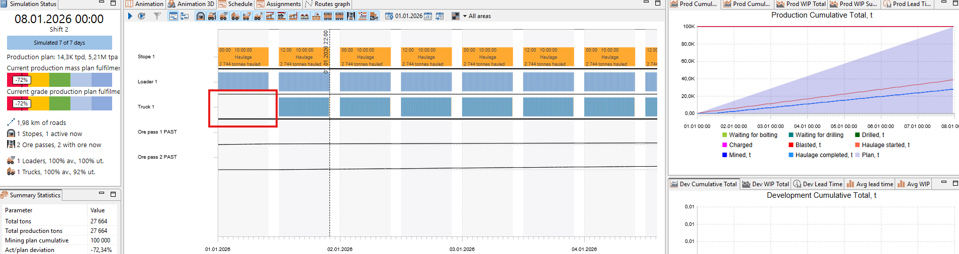
We run the simulation again and open the schedule to check how the equipment is assigned. The LHD is working, and the truck also receives assignments later in the run, but Truck 1 is not scheduled during the first shift. This happens because the default planning mode creates equipment tasks shift by shift. At the beginning of the first shift, Ore pass 1 is still empty, so MineTwin does not yet create a truck haulage task from this transfer point. We correct this by changing the haulage scheduling mode.

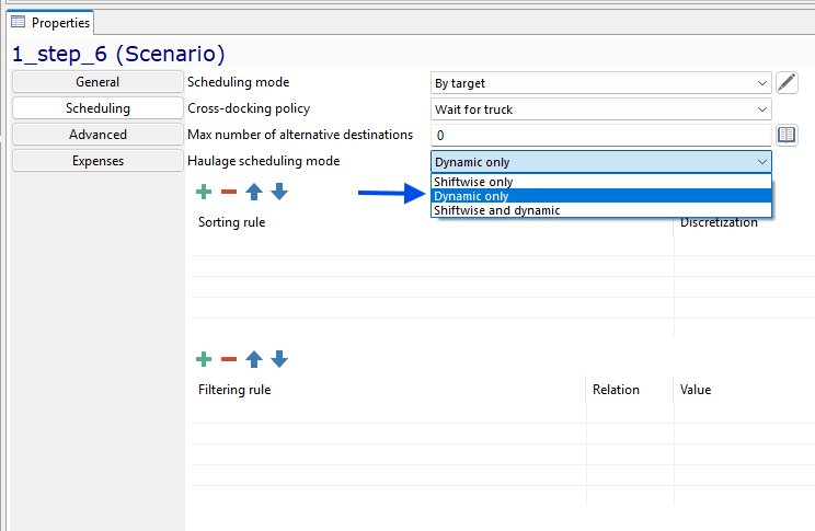
We return to the scenario scheduling settings and change Haulage scheduling mode to Dynamic only. In this mode, the dispatcher keeps looking for available haulage tasks during the simulation instead of only preparing tasks for the whole shift in advance. This means the truck can receive a task as soon as material appears in Ore pass 1.

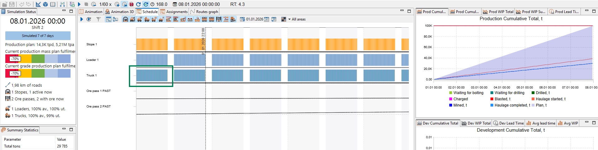
We run the simulation again and review the schedule. Now Truck 1 receives work during the first shift, so the dynamic dispatcher is creating truck haulage tasks as soon as material becomes available in Ore pass 1. However, the production plan is still not fulfilled. The status panel and production chart show that the scenario remains behind the target.

Download the intermediate scenario after adding the second ore pass and truck haulage

In this section, we extend the material flow beyond Ore pass 2. The truck now has a destination, but the scenario still needs an onward handling chain for the material collected at the second ore pass.

We add a conveyor arc, connect Ore pass 2 to that conveyor, create the conveyor object, and then add the skip hoist with its input buffer and final storage. After the objects are connected, we review the result in 3D and run the full chain to check that material can move through the downstream path.

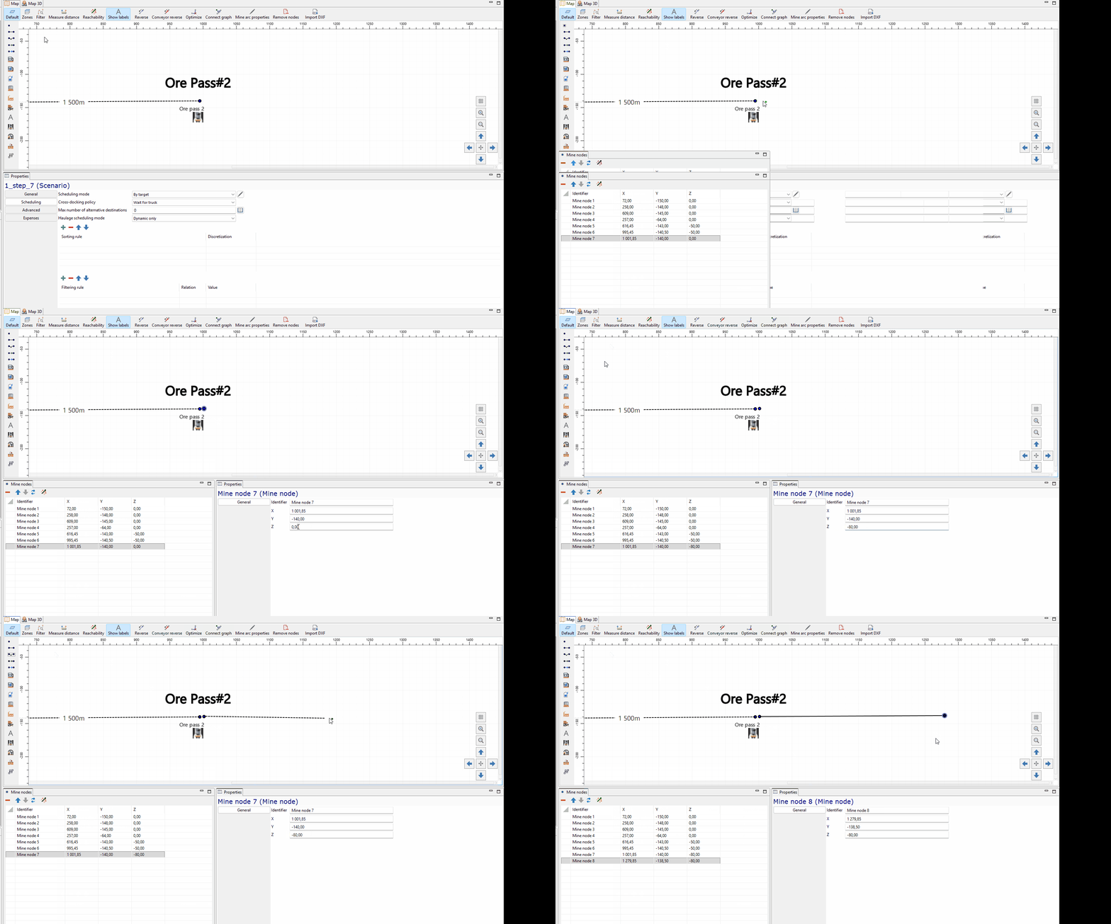
We draw a new line from the area near Ore pass 2 to create the third leg of the material flow. At this point, the new geometry is still just a mine arc, so we will change its type before using it as a conveyor.

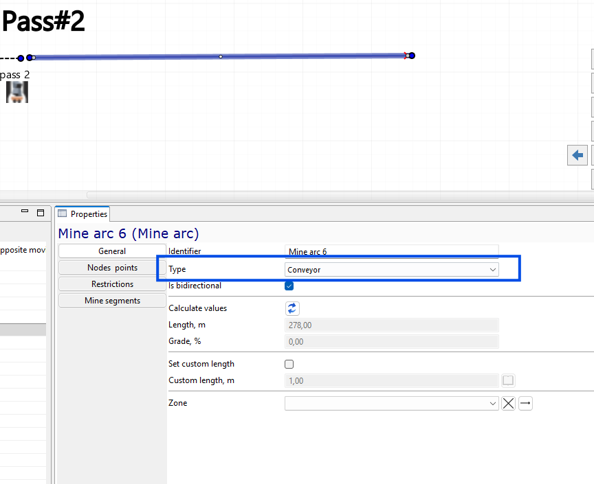
We select the new mine arc and change its type to Conveyor. This tells MineTwin that the arc should be used by conveyor equipment rather than by mobile haulage equipment.

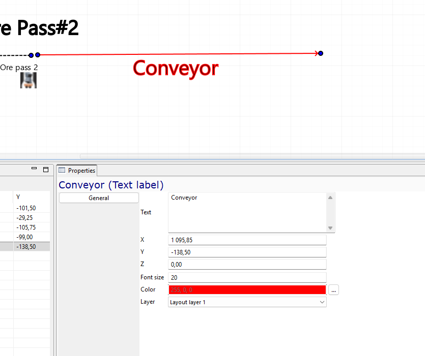
We add a red Conveyor label along the new arc. The label is a visual annotation for the training map, and it makes the downstream material flow easier to follow during the demonstration.

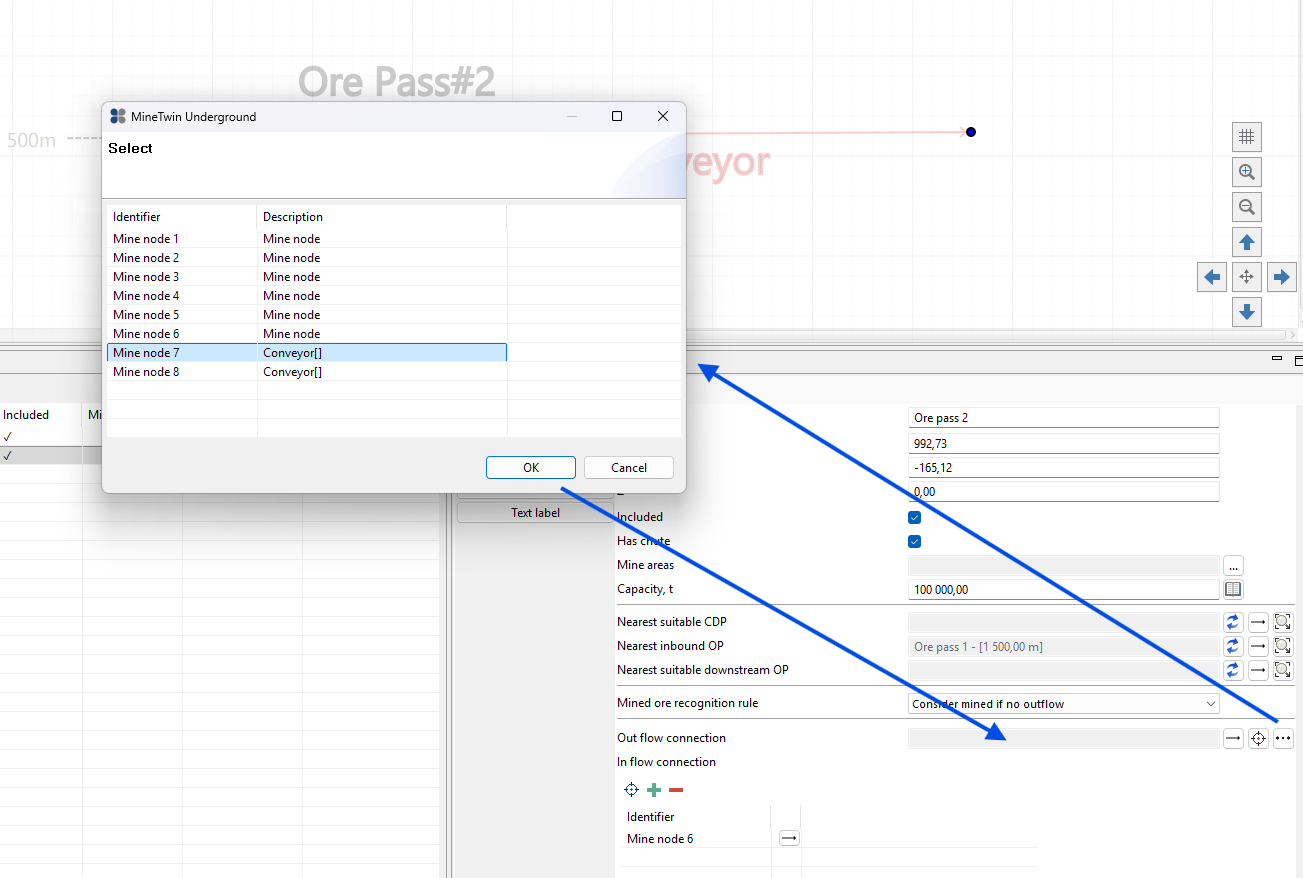
We select Ore pass 2 and assign its outbound connection to the conveyor input node. This defines where material leaves the second ore pass and enters the conveyor line.

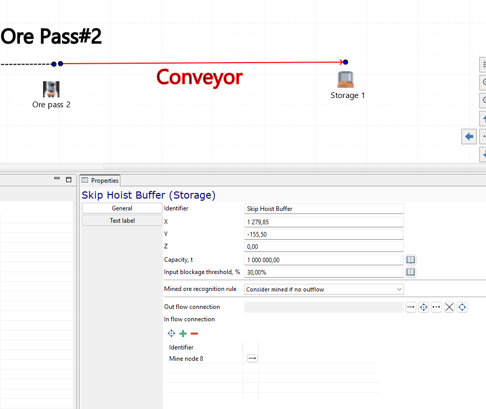
We create Skip Hoist Buffer at the end of the conveyor and connect its inflow to the conveyor output node. This storage object works as the intermediate buffer between the conveyor and the skip hoist.

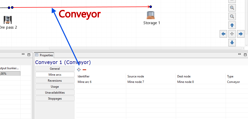
We create Conveyor 1 and associate it with the conveyor-type mine arc. The conveyor object now knows which map arc it operates on, including the source node and destination node of that conveyor segment.

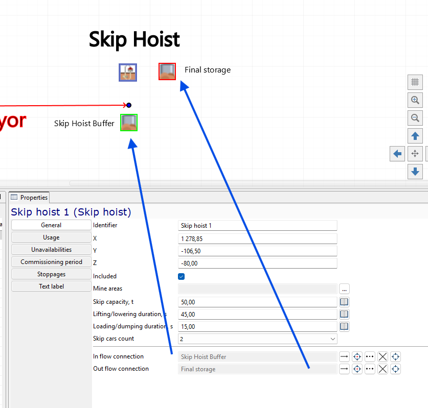
We create Skip hoist 1 and connect its inflow to Skip Hoist Buffer. Then we create Final storage and connect the skip hoist outflow to it. This completes the downstream chain from the second ore pass through the conveyor and skip hoist to the final storage.

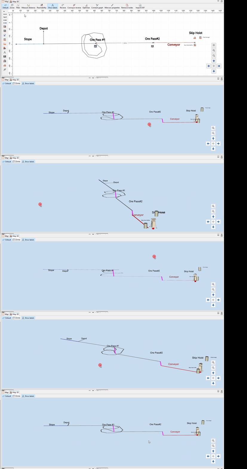
We switch to the 3D view and review the scheme we have built. At this point, we are only checking the geometry and object placement visually. The 3D view helps us confirm that the stope, depot, ore passes, conveyor, skip hoist buffer, skip hoist, and final storage are arranged as expected.

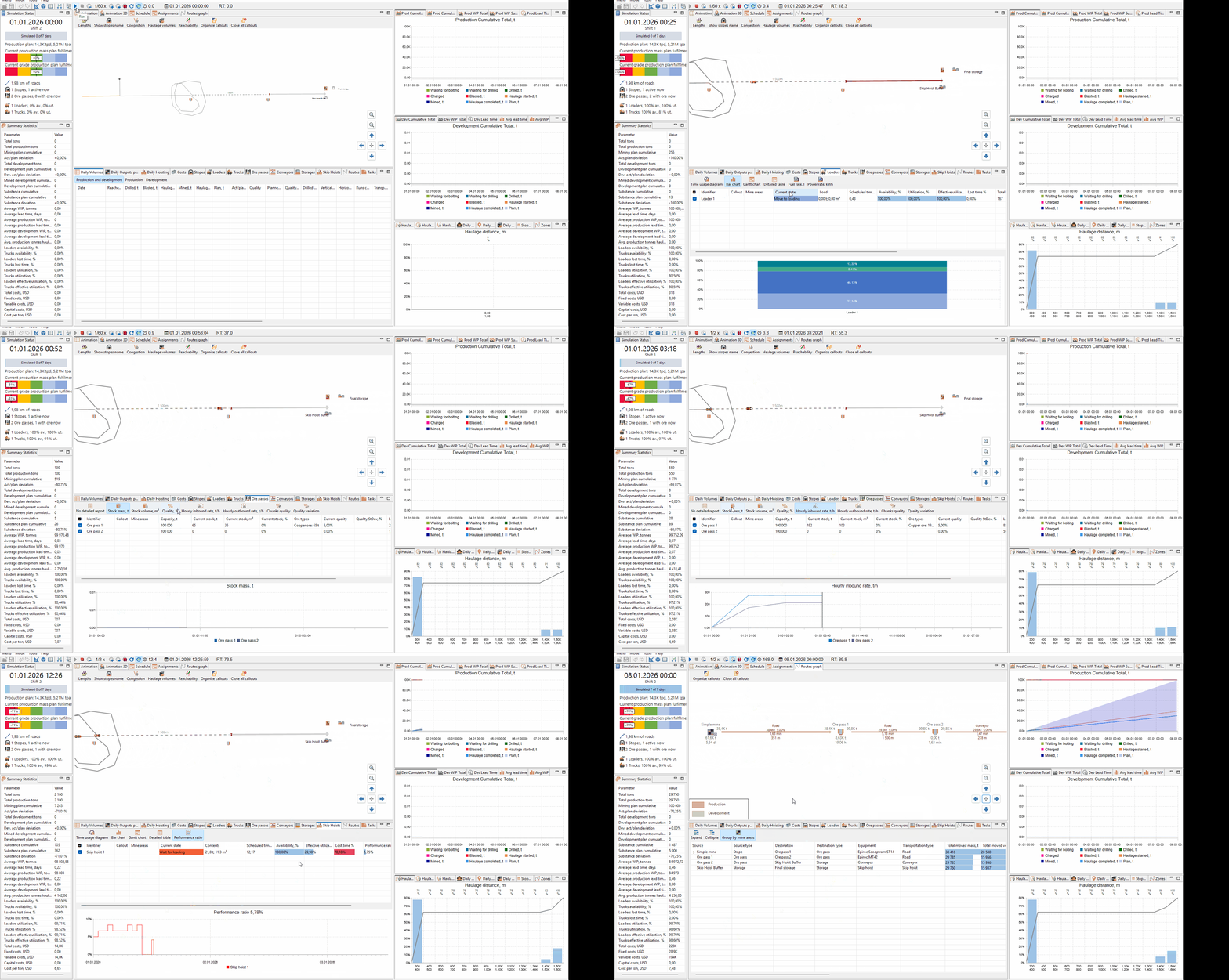
We run the simulation again after adding the conveyor, skip hoist, and final storage. This run checks the complete material flow from the stope to the first ore pass, then by truck to the second ore pass, through the conveyor to the skip hoist buffer, and finally through the skip hoist to the final storage. The animation and result panels help us confirm that the downstream objects are connected and that material can move through the full chain.

Download the final scenario for the first training section