Add drilling and charging

In this section, we will change the block logic from direct haulage to a more complete drill-and-blast mining cycle. We will update the block advancement type, review the new drilling-related parameters, apply the same setup to the second block, and run the simulation to see what is still missing.

This step is important because the previous scenario allowed ore to be hauled without modeling preparation work. After this change, MineTwin will require drilling and charging before the blocks can move to later mining stages.

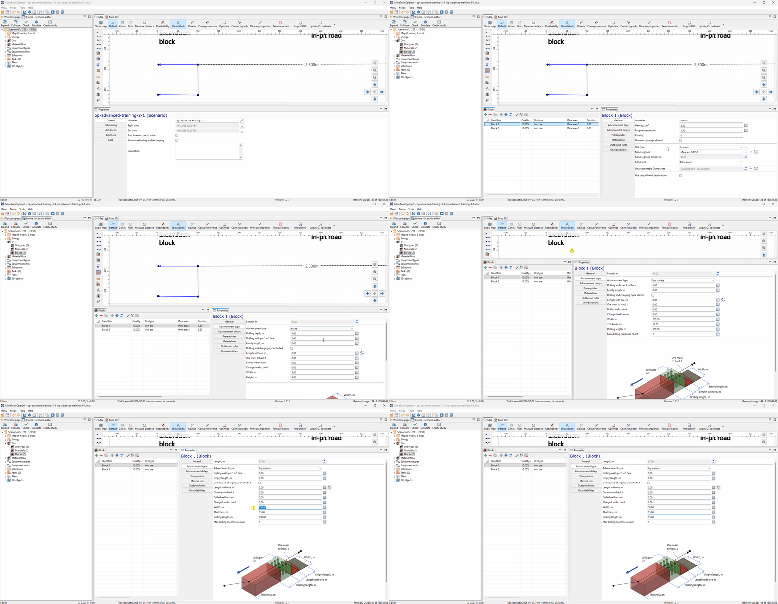
We change the advancement type for the block to Top surface and start adjusting the parameters required for the drill-and-blast cycle. According to the MineTwin OpenPit block setup, this advancement type models vertical drilling, charging, and loading out the block in sections of a specified length.

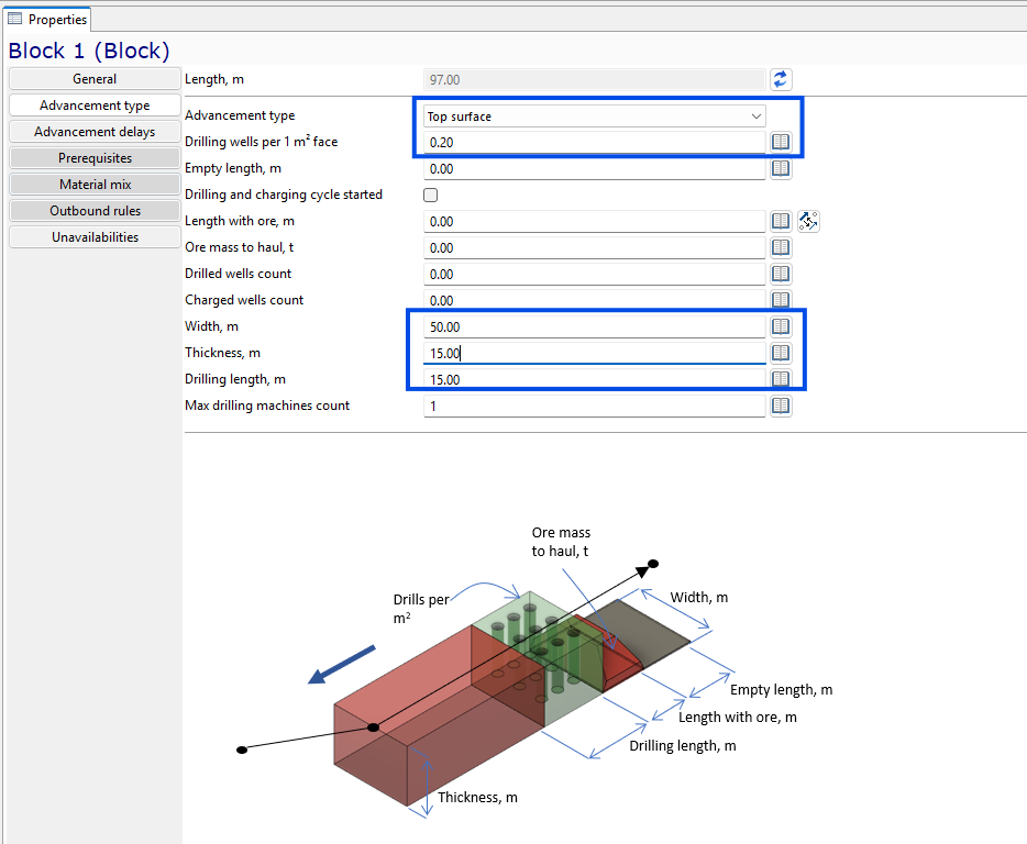
We set the Top surface advancement parameters highlighted in blue. These include drilling wells per square meter of face, width, thickness, and drilling length. Together, these values define the drilling requirement that MineTwin will use before the block can advance to charging and haulage.

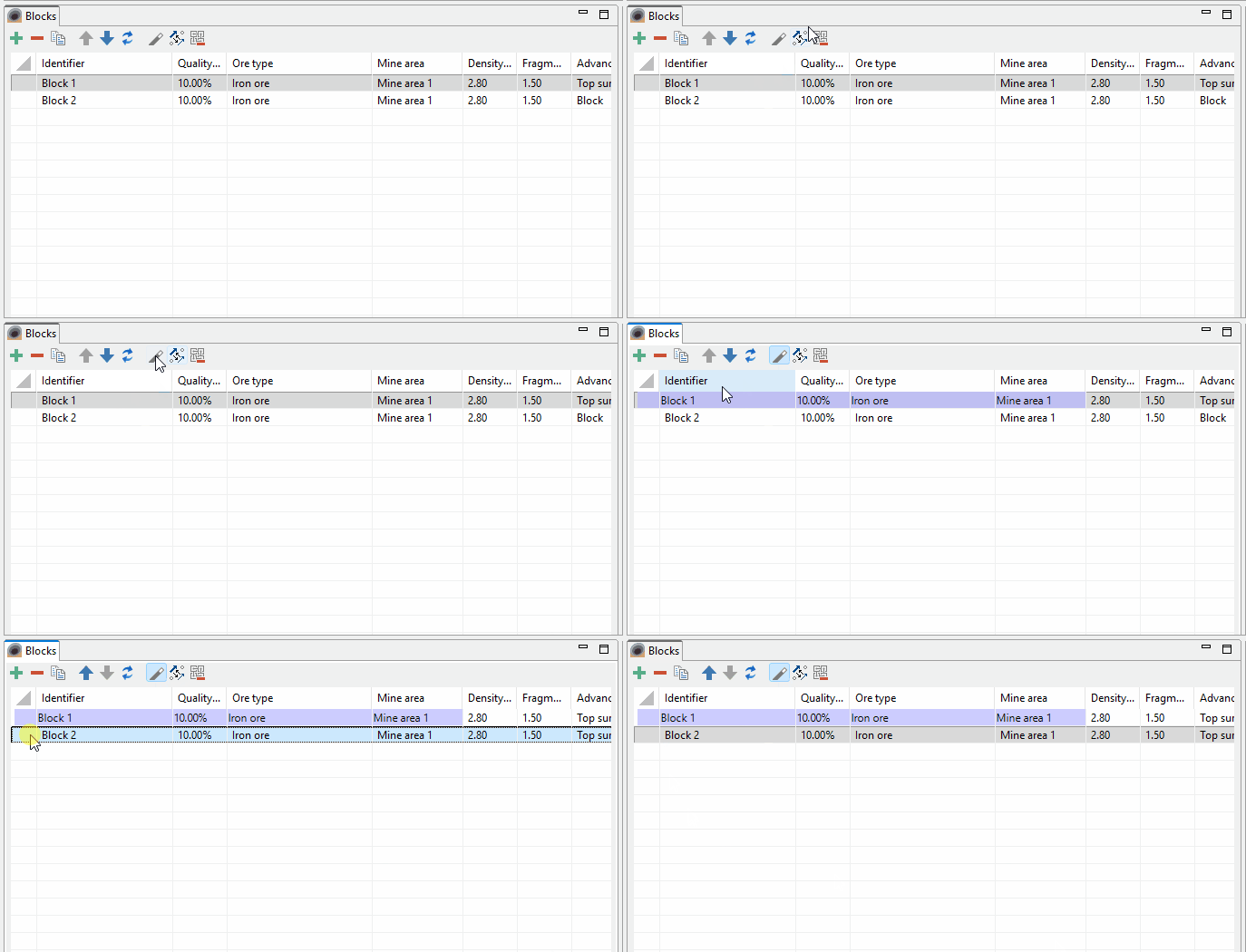
We use the first block as a template and apply its advancement type settings to the second block. This keeps both ore blocks consistent, so the simulation treats them as blocks that require drilling and charging before material can be hauled.

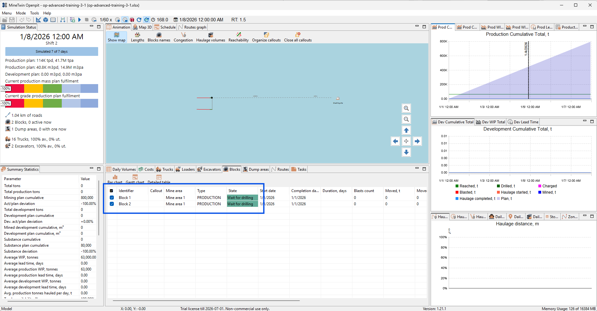
We run the simulation after adding the drilling and charging requirement. The result shows both blocks in the Wait for drilling state, while production remains at zero. This confirms that the new block logic is active, but the scenario still has no drilling and charging equipment to perform the required preparation work.

Download scenario

In this section, we will add the equipment needed to perform the drilling and charging steps introduced in the previous section. We will import drilling machine and charger types from the library, create a depot node for this equipment, add equipment units, and rerun the simulation.

The purpose of this section is to close the gap revealed by the previous run. Once drills and chargers are available, the blocks should be able to move from Wait for drilling through drilling and charging states.

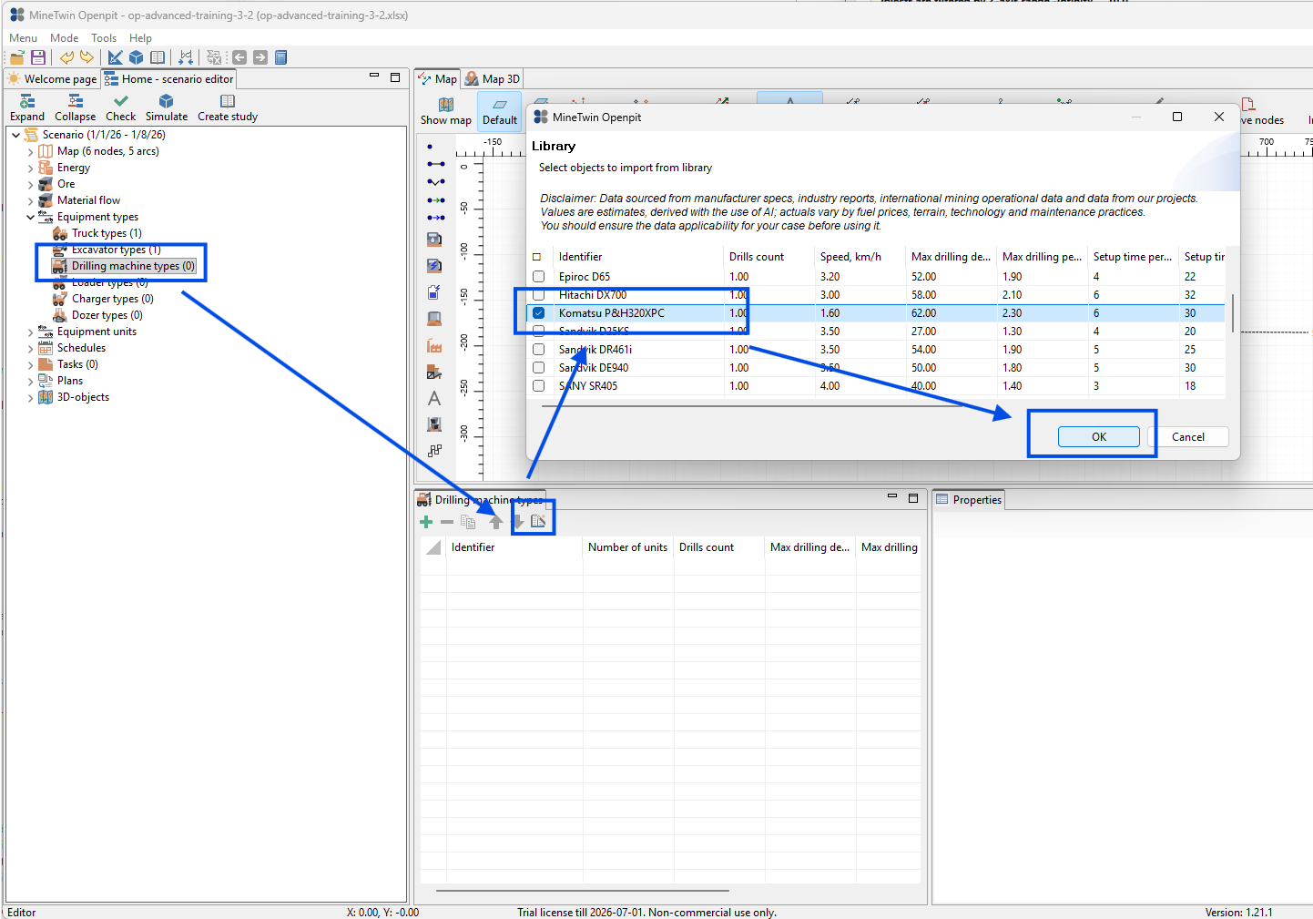
We add a drilling machine type from the MineTwin library. In this example, we select the Komatsu P&H320XPC drilling machine type, and its parameters are populated from the library for use in the scenario.

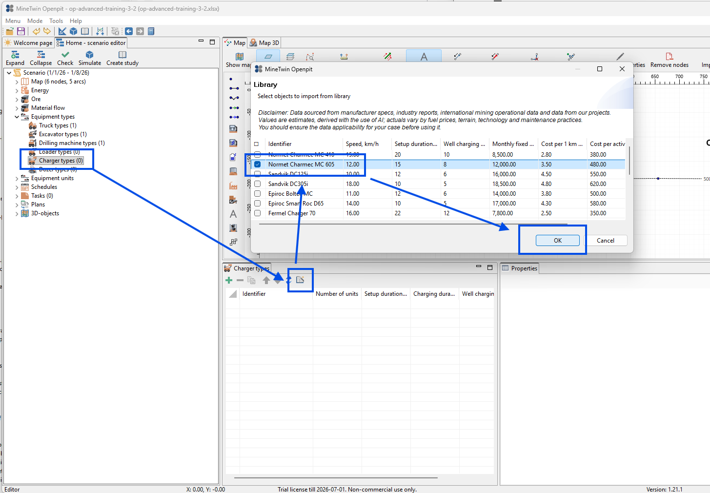
Next, we add a charger type from the library. We select the Normet Charmec MC 605 charger type, which provides the charging-related parameters used later by the charger unit.

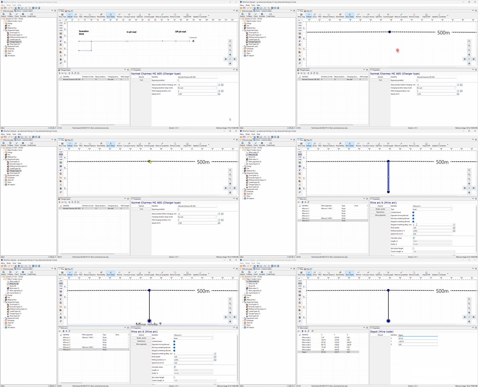
We add a depot node on the road network for the drilling machine and charger. This node will be used as the initial position for the new equipment units, similar to how base nodes were used for trucks and excavators.

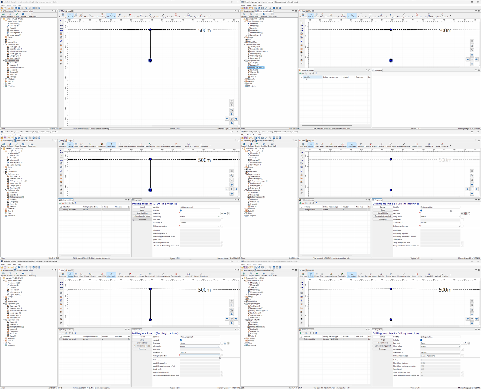
We create one drilling machine unit based on the imported drilling machine type. The unit is assigned to the depot node, so MineTwin knows where it starts before traveling to the blocks that require drilling.

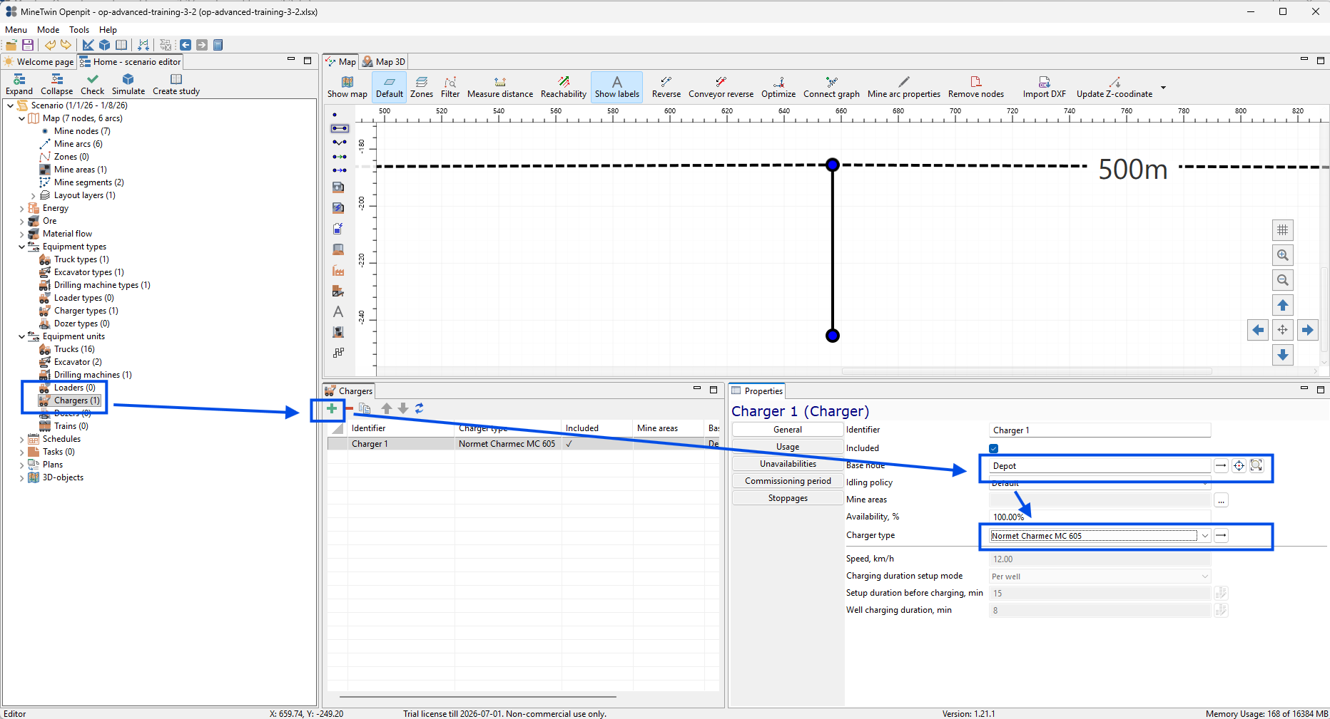
We create one charger unit based on the imported charger type. The charger is also assigned to the depot node and will be used after drilling is completed to charge the drilled wells.

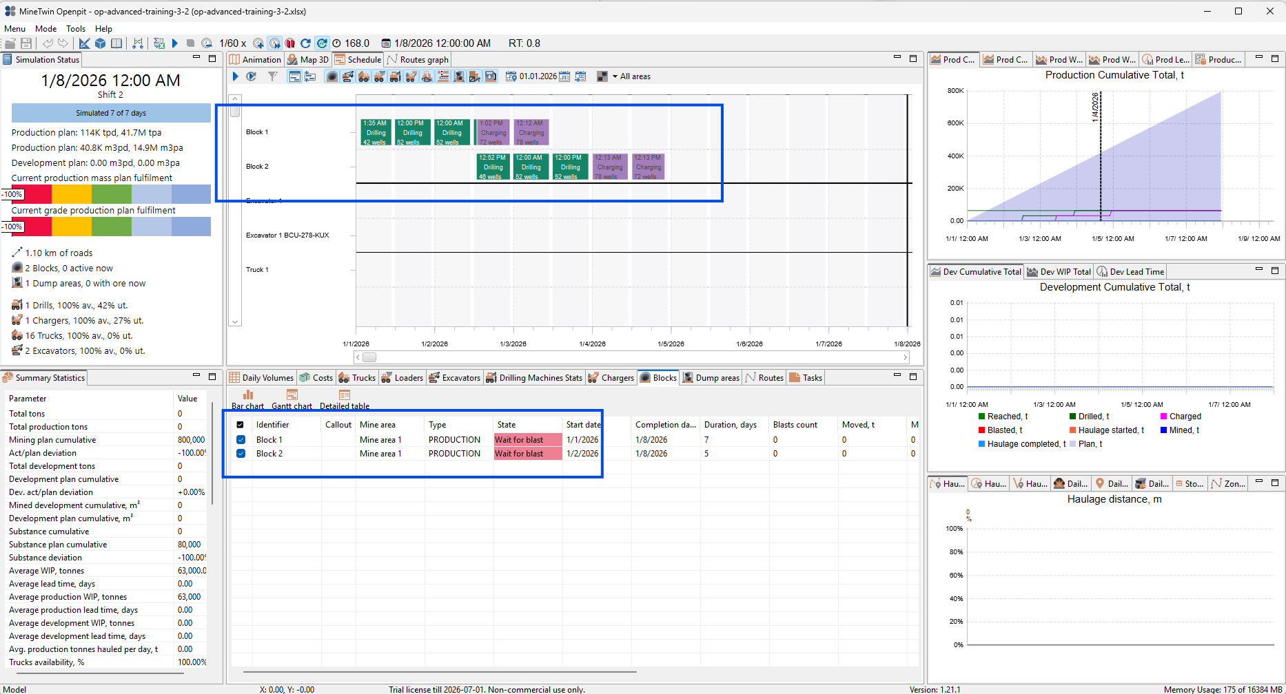
We run the simulation again to check whether the new equipment can perform the required preparation work. The Gantt chart shows drilling and charging operations for both blocks, and the block table shows that the blocks progress to the Wait for blast state. This confirms that drilling and charging are now modeled, but blasting still needs to be configured before the full mining cycle can continue.

Download scenario

In this section, we will add blast periods and complete the basic drill-blast-haul cycle. We will first define when blasting is allowed, then run the simulation to see how blocks move through drilling, charging, blasting, and haulage.

After that, we will adjust the charging duration to a more realistic value for the current block setup. This helps us refine the timing of the preparation stages before we extend the scenario further.

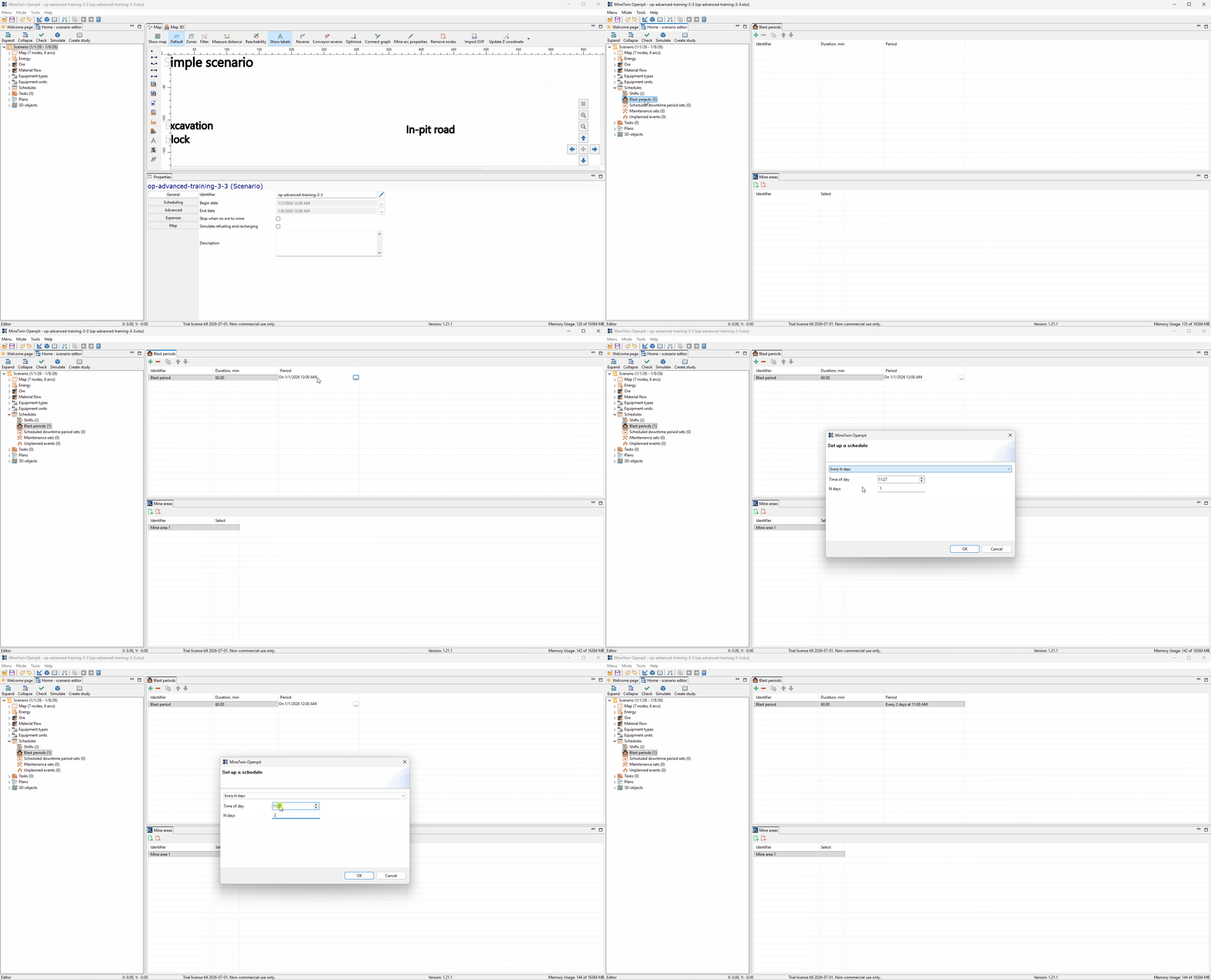
We add blast periods to the schedule every other day at 11:00 AM. These periods define when charged blocks are allowed to be blasted, so the simulation can move blocks from Wait for blast to the next mining stage.

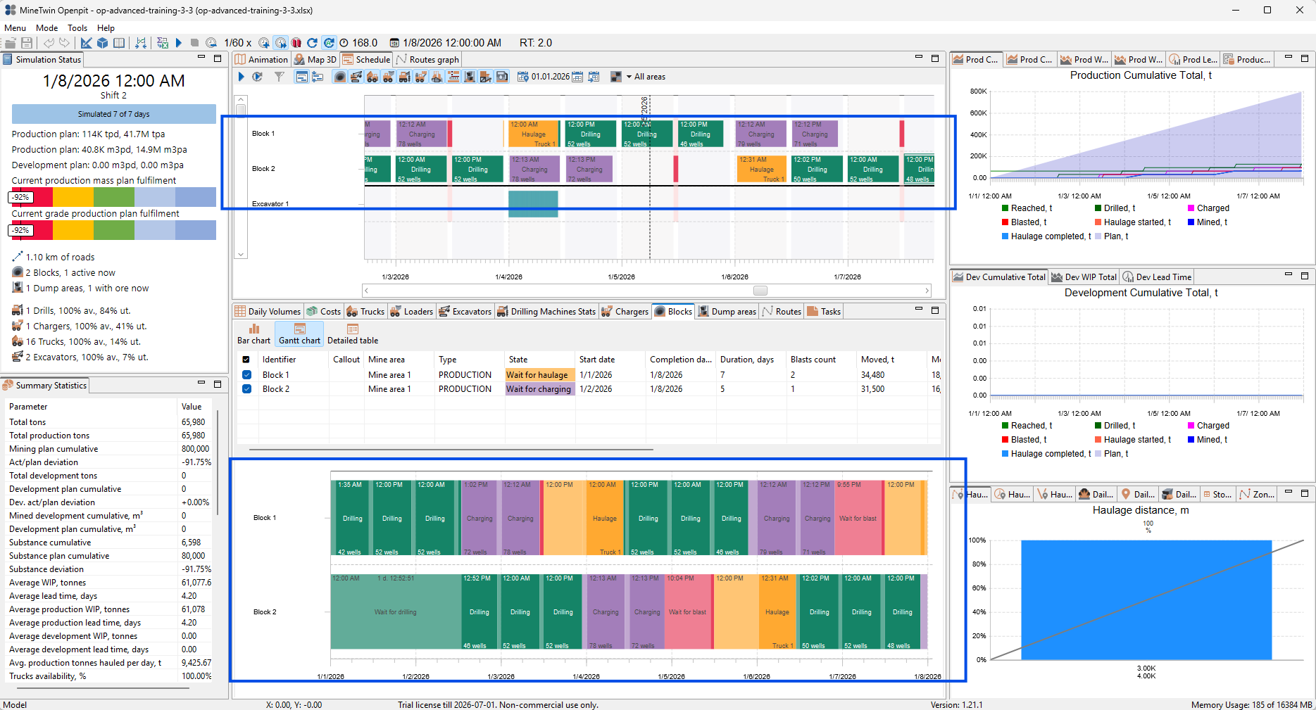
We run the simulation and review the full mining cycle on the Gantt chart. The chart now shows drilling, charging, wait for blast, blast events, and haulage for the blocks. The block table confirms that the blocks can progress beyond preparation work, although the production result is still far below the 800,000 t target.

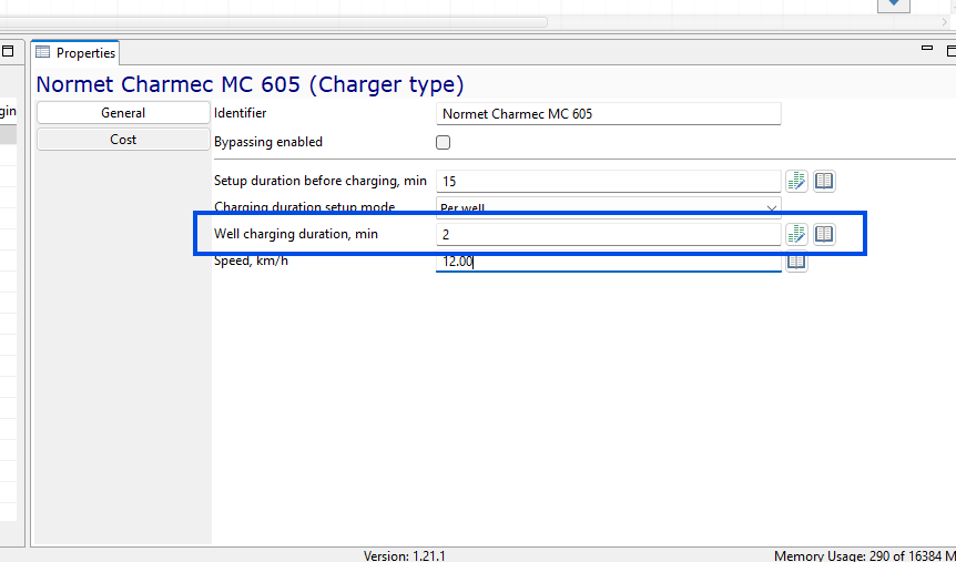
We adjust the well charging duration for the charger type to 2 minutes per well. This shortens the charging stage and makes the charger performance more appropriate for the current block configuration.

Download scenario

In this section, we will expand the scenario from two blocks to four blocks and extend the simulation period to one month. We will add geometry for two additional block locations, create the corresponding mine segments, copy the existing blocks, and assign the copies to the new segments.

After the model is extended, we will run the simulation and use the analytical views to understand how material moves through the drill-and-blast-haul cycle. We will focus on state changes, WIP, lead time, and the detailed state history for an individual block.

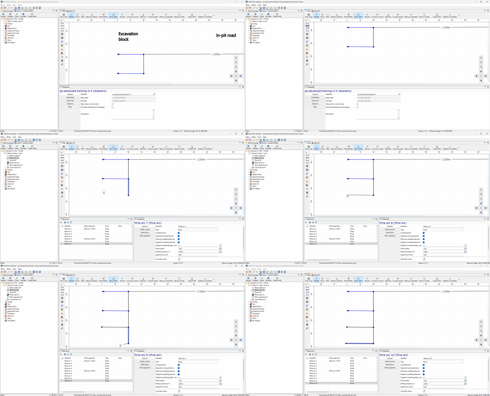
We draw the geometry for two additional blocks on the map. These new lines extend the mining layout and prepare the road network geometry that will later be linked to new mine segments.

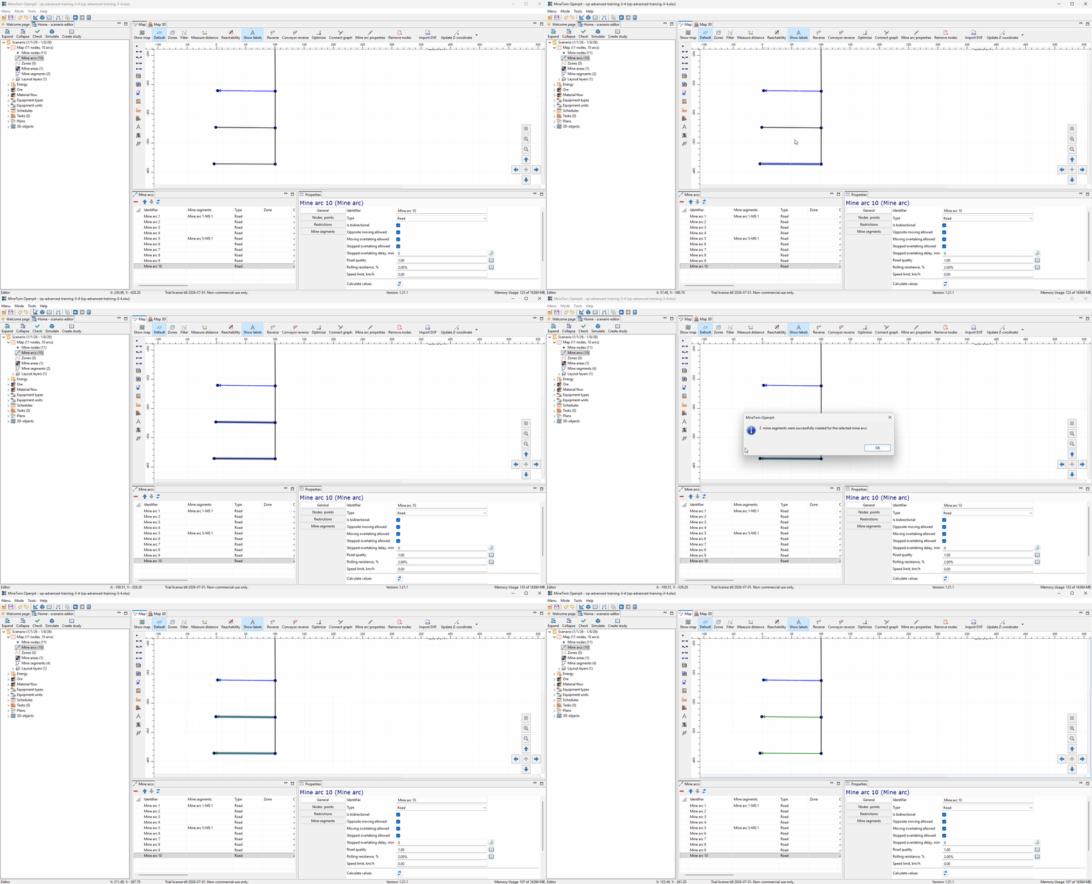
We create mine segments for the new block locations. A mine segment defines the directed polyline that represents where a block is located in the model, so it connects the block logic to the map geometry.

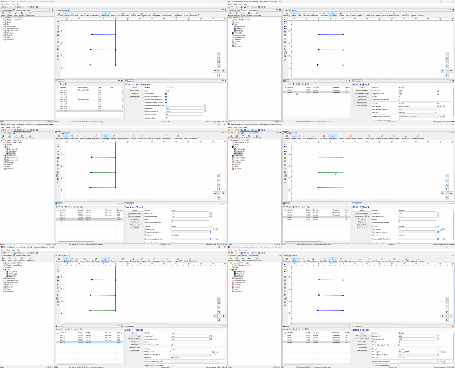
We copy the already configured blocks and assign the new copies to the new mine segments. This lets us reuse the ore type, mine area, density, and advancement settings that were already prepared for the first blocks.

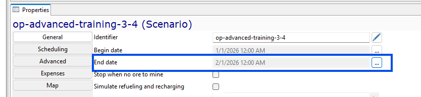
We extend the scenario end date to February 1, 2026. This gives the simulation enough time to process the larger set of blocks and evaluate the mining cycle over a full month.

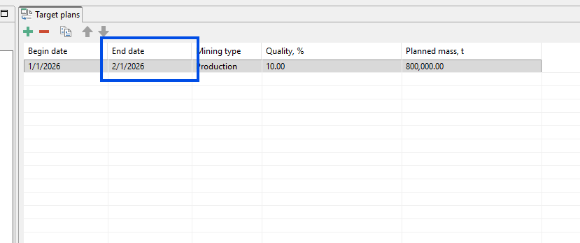
We extend the production plan to the same end date. The target remains 800,000 t with 10% quality, but the planning period is now aligned with the longer simulation horizon.

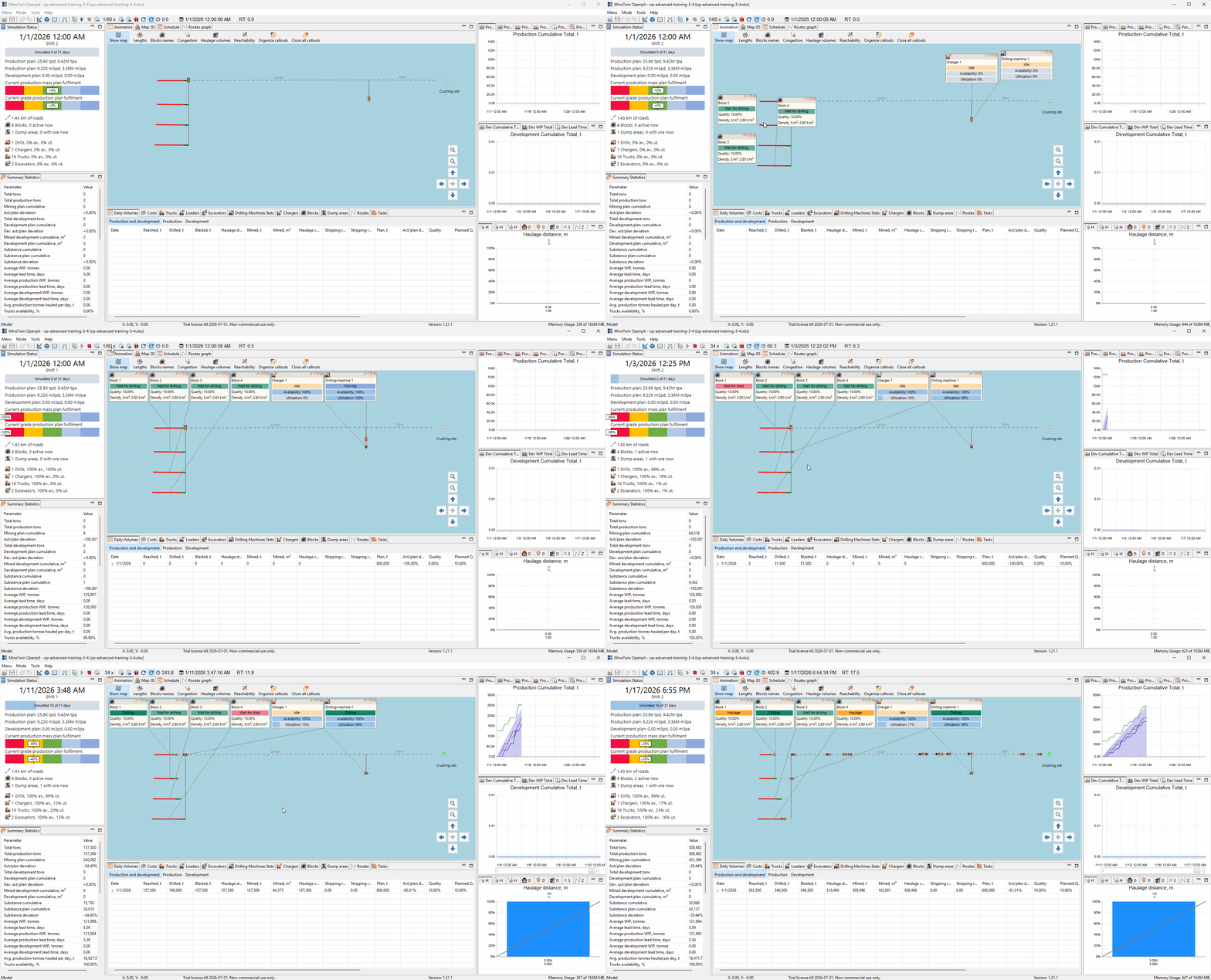
We run the simulation and use callouts on the animation map to inspect the current state of blocks and equipment. The callouts show blocks moving through drilling, charging, waiting for blast, and haulage, while equipment callouts show availability and utilization during the run.

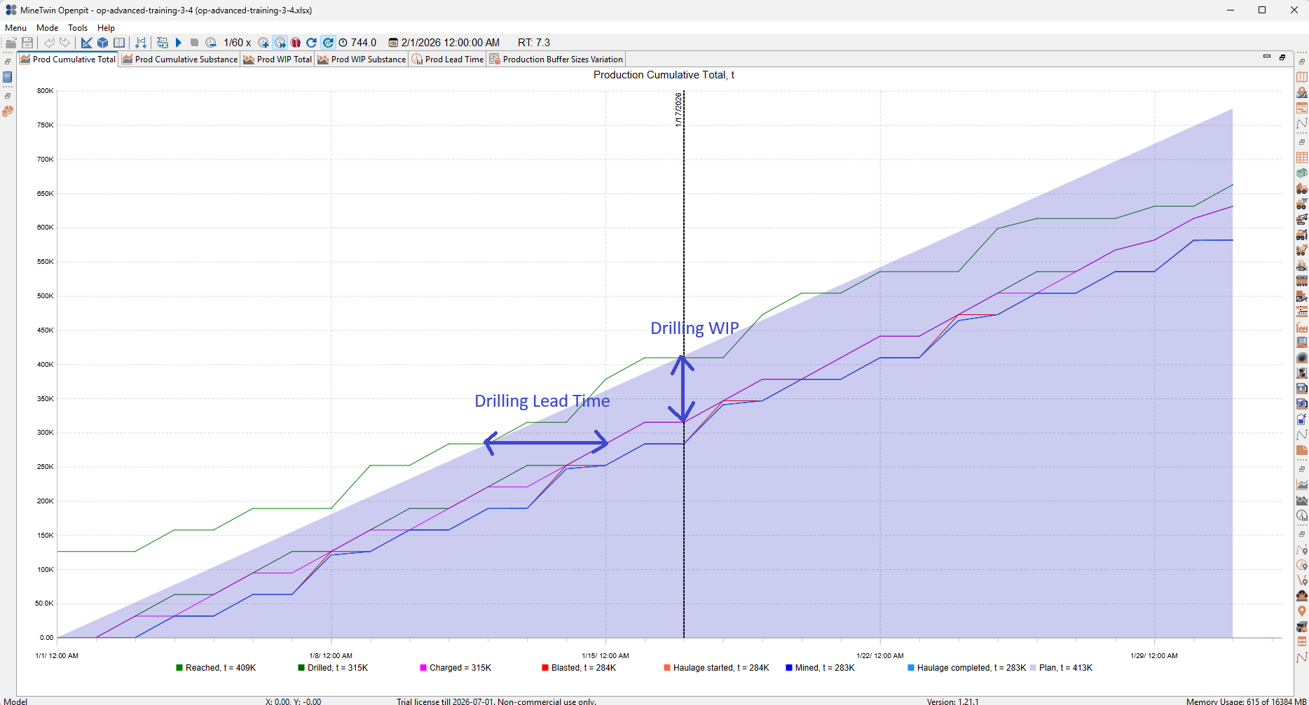
We review the Production Cumulative Total chart to compare how much material has passed each mining stage over time. The vertical gap between stage lines shows WIP, while the horizontal distance between lines shows lead time for material moving through the process.

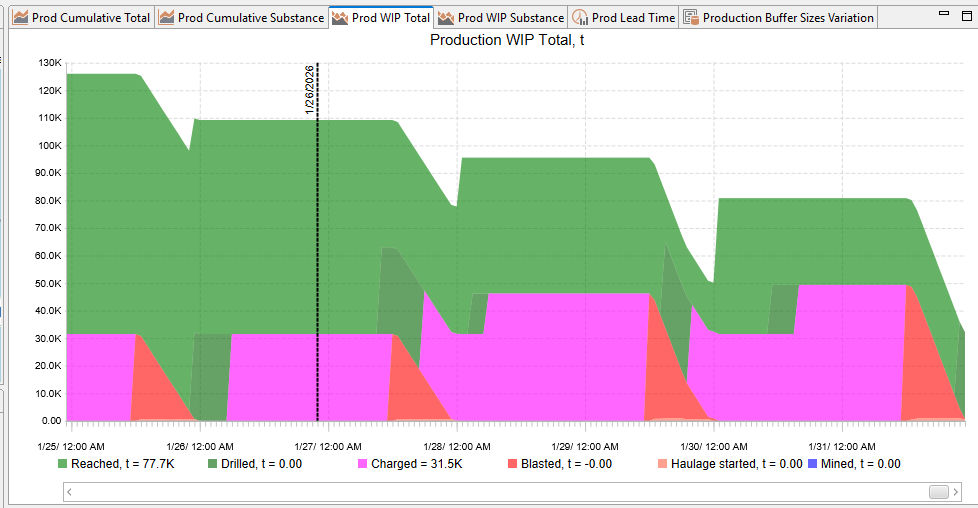
We open the Production WIP Total diagram to see where material accumulates between stages. This view helps identify whether the scenario is building queues before drilling, charging, blasting, or haulage.

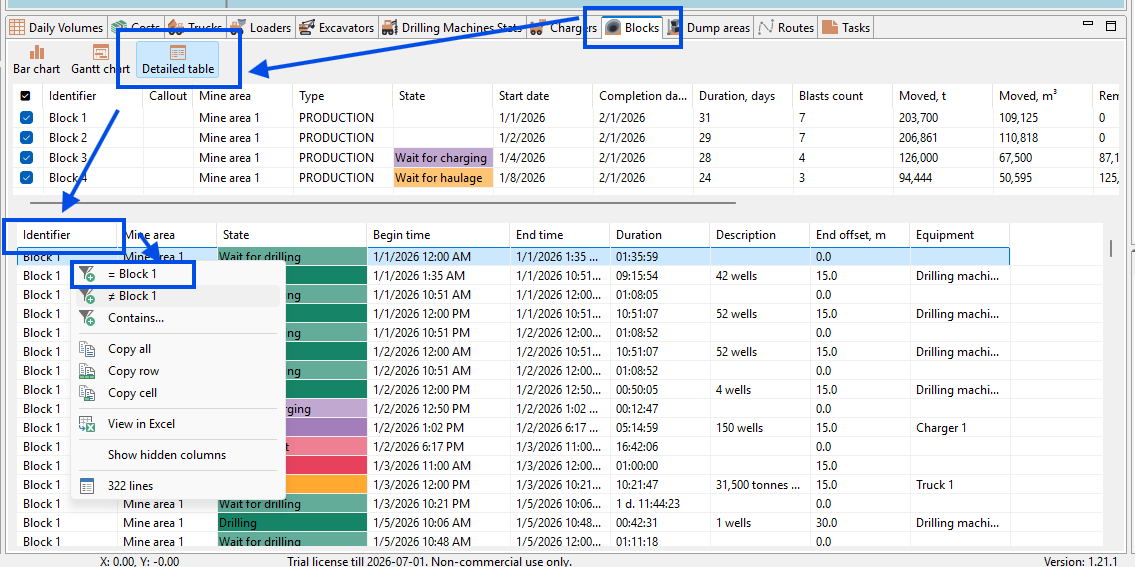
We open the detailed block states table and filter it by Block 1. This gives us the exact sequence of state periods, including begin time, end time, duration, and the equipment involved in work on the block, so we can trace how one block moved through the mining cycle.

Download scenario

In this section, we will use the Constraint Analysis study to identify what prevents the scenario from reaching the production target. The study creates a set of targeted scenario modifications and compares their results with the baseline scenario.

This is a diagnostic step rather than a final planning decision. We use it to understand which limitation has the strongest effect on mined tons, then apply the most practical change to the original scenario and verify the result with a new simulation run.

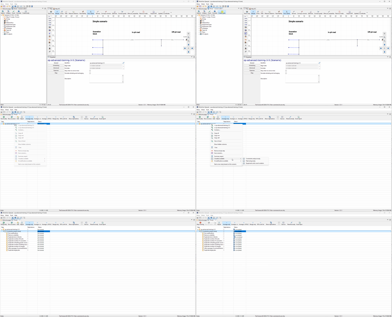
We start a Constraint Analysis study from the current scenario. MineTwin generates a branch with the baseline case and a set of modification scenarios, such as duplicating equipment, removing variability, duplicating block tons, or changing other limiting conditions.

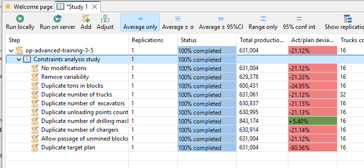
We review the completed study table and compare the effect of each modification on production. The result shows that duplicating the number of drilling machines gives the strongest improvement: production increases to 843,174 t and the act/plan deviation becomes +5.40%, while the baseline remains at 631,004 t and -21.12%.

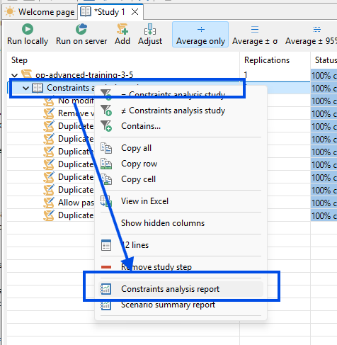
We open the Constraints analysis report from the study context menu. The report gives a more readable summary of the same comparison, so we can use it to explain which constraint has the greatest impact.

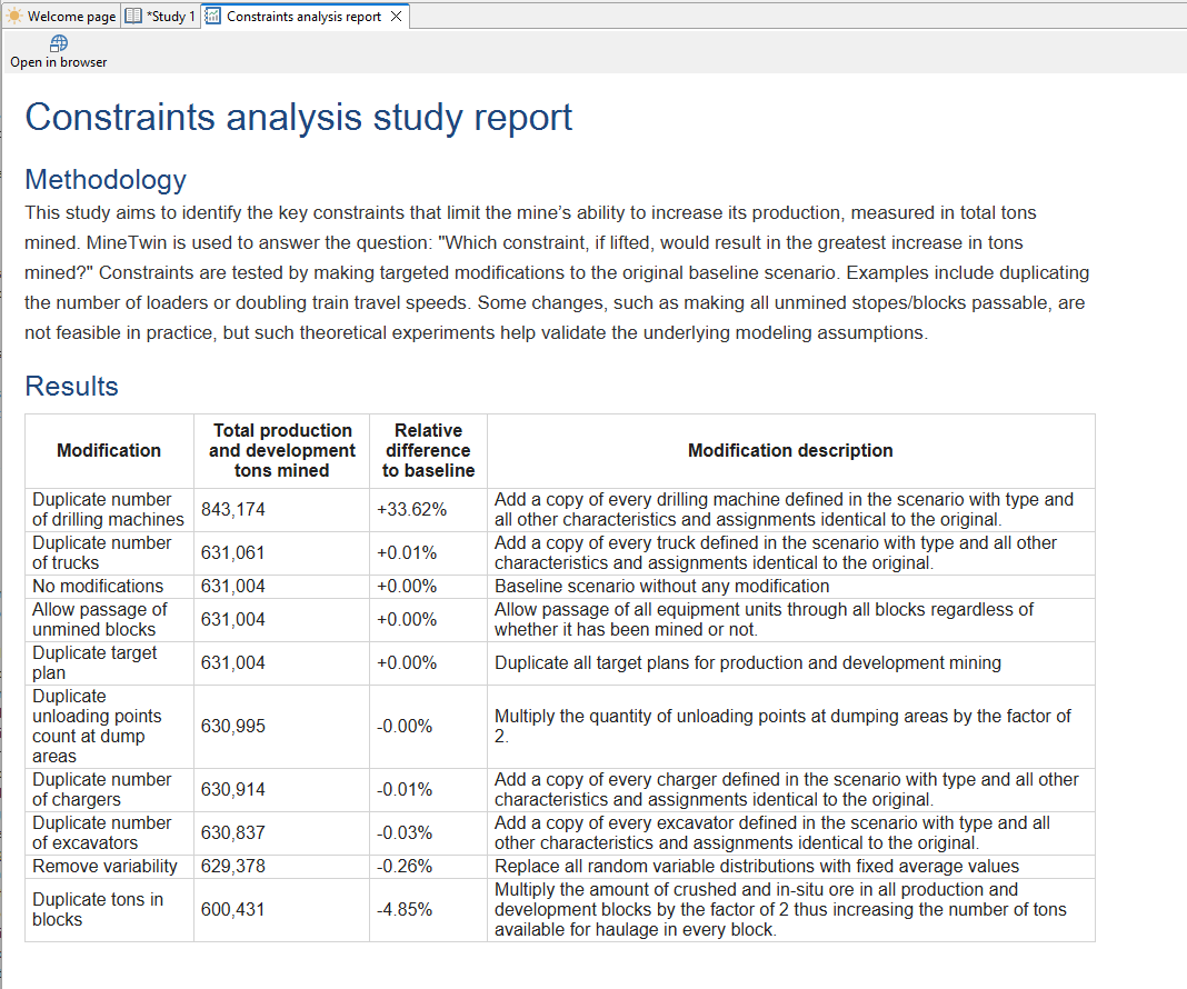
We review the report methodology and results table. The report confirms that the study tests targeted modifications to answer which constraint would increase production the most if it were lifted, and it identifies drilling machines as the leading constraint in this scenario.

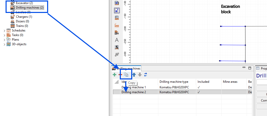
Based on the study result, we add a copy of the existing drilling machine. This gives the scenario two drilling machines with the same type and settings, so drilling capacity is increased without changing the rest of the mining logic.

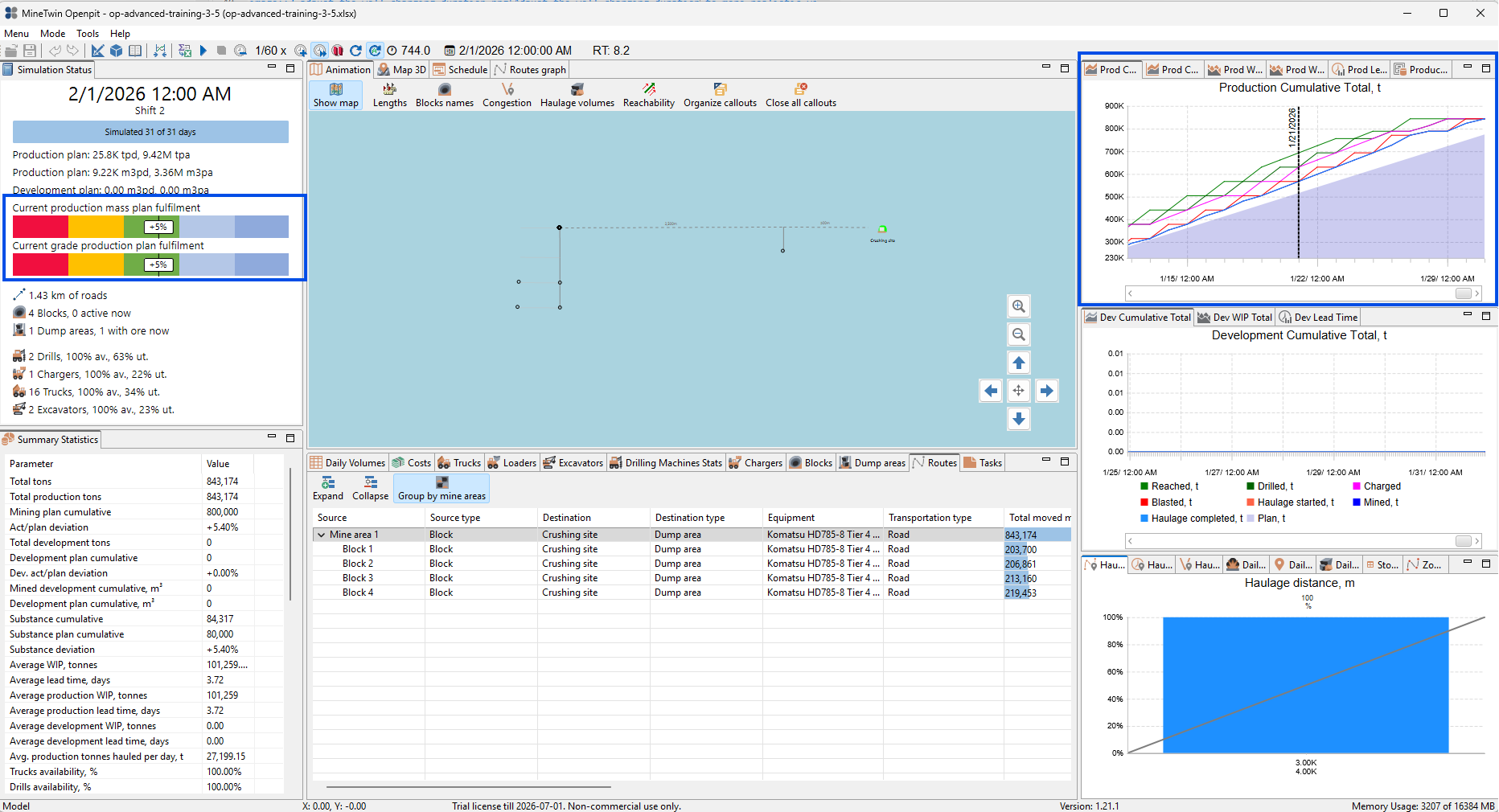
We run the simulation again after adding the second drilling machine. The scenario now reaches the monthly production plan with 843,174 t mined and a +5.40% production plan deviation, confirming that drilling capacity was the main practical constraint in this setup.

Download scenario