Add stockpiles and the second leg of transportation

In this section, we will prepare the off-pit geometry for stockpiles and the second leg of transportation. We will rename the area label, draw additional road geometry, reconnect the existing Crushing site dump area, verify node elevations, and create an off-pit zone for later statistics.

This geometry will become the physical layout for intermediate stockpiles between the pit and the final crushing site. It also gives us a separate off-pit area where we can later analyze route speeds and other movement indicators independently from the in-pit haul road.

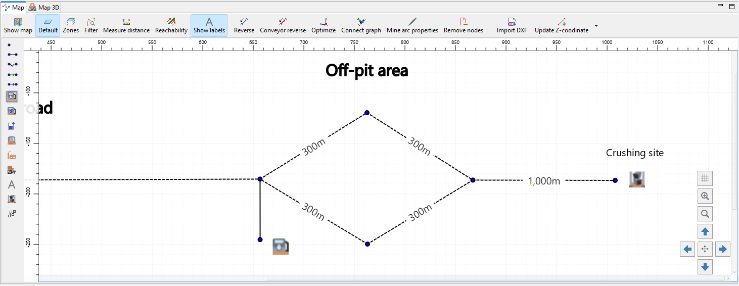
We change the text label from Off-pit road to Off-pit area. Then we draw the stockpile road geometry in the off-pit area and assign the custom lengths shown on the map. The new geometry creates two alternative 600 m branches through the future stockpile area, with each branch consisting of two 300 m sections. It also adds a 1,000 m connection toward the Crushing site.

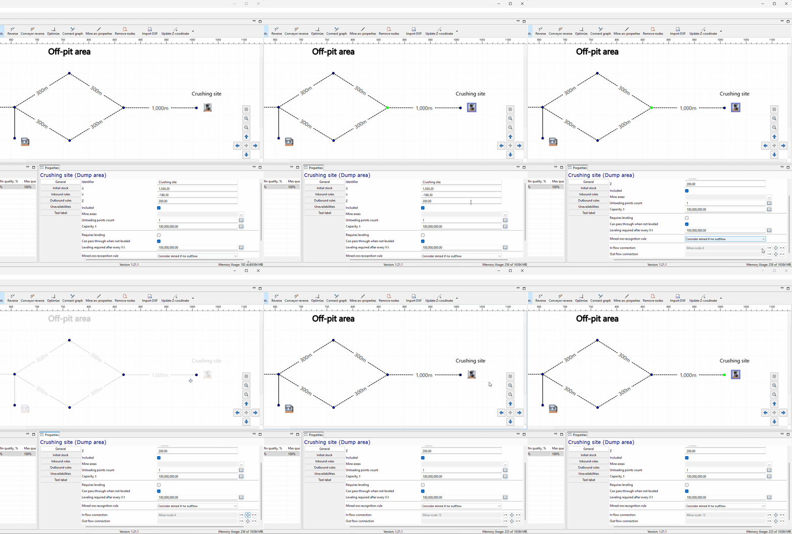
We reassign the existing Crushing site dump area to the new mine node at the end of the off-pit connection. This keeps the same dump area object, but moves its connection point to the updated road geometry.

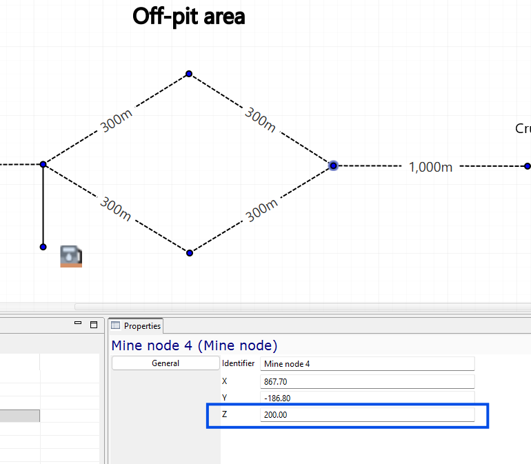
We check the Z coordinates for the newly drawn nodes and set them to 200 m. These nodes are located on the surface level, and correct elevations are required for proper gradient calculations.

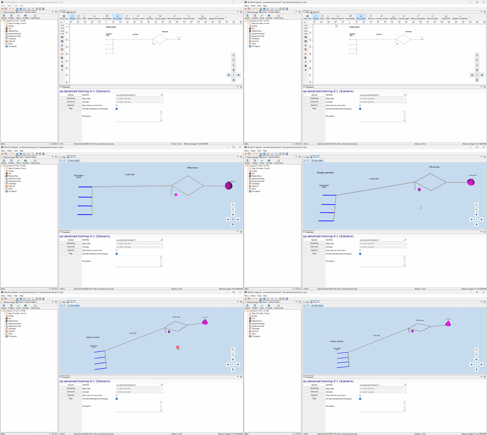
We review the geometry in the 3D view to confirm that the new off-pit nodes sit at the expected elevation. This visual check helps us catch incorrect Z values before using the geometry in simulation.

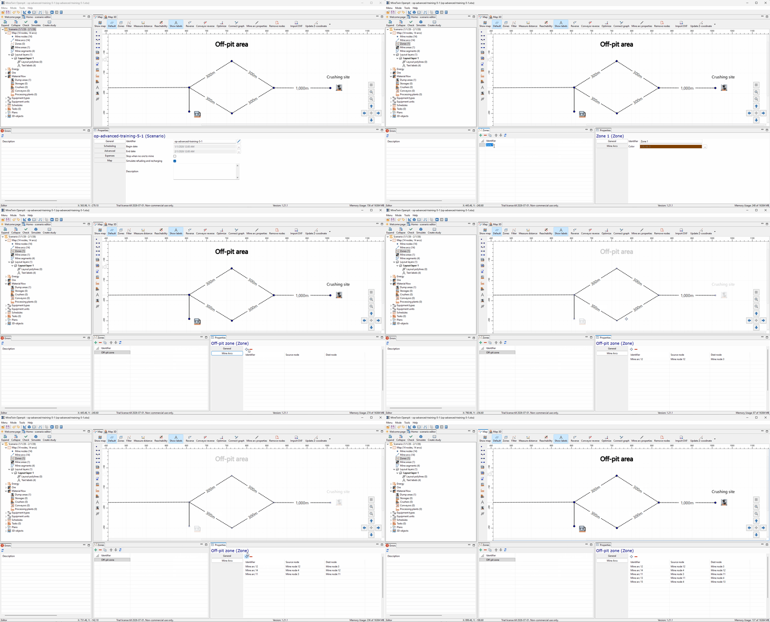
We create an Off-pit zone and assign the newly added off-pit mine arcs to it. This zone will let us analyze movement indicators for the off-pit part of the haulage network separately from the in-pit road.

Download scenario

In this section, we will add two intermediate stockpiles to the off-pit area. We will first create a high-grade stockpile and route all current ore to it, then add a low-grade stockpile for ore with lower quality.

Both stockpiles are modeled as dump areas. This allows trucks to unload material into them, while inbound quality rules determine which stockpile can accept each ore flow.

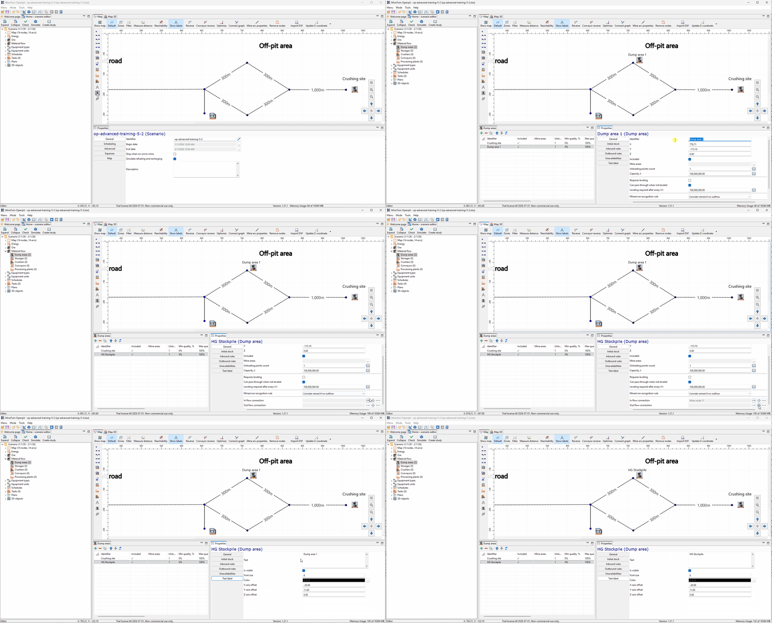
We add a new dump area named HG Stockpile on the upper branch of the off-pit geometry. We connect both its inflow and outflow to the top stockpile node, so the stockpile can receive ore from the pit and later serve as a source for the next transportation leg.

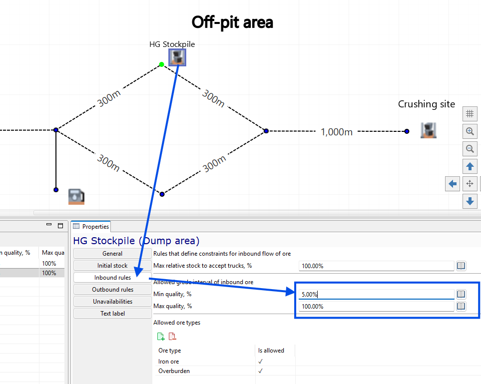
We set the inbound quality rule for the HG Stockpile. The stockpile accepts material with quality from 5% to 100%, so it is used for high-grade ore.

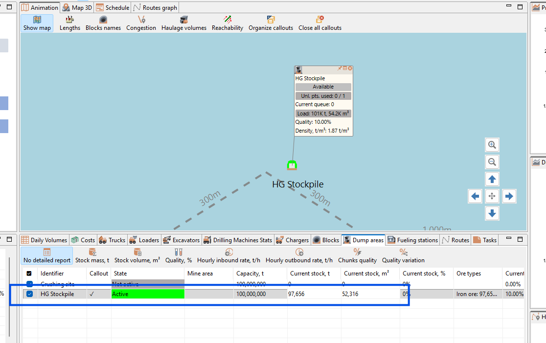
We run the simulation and review the stockpile state. All currently mined ore is routed to the HG Stockpile, and the dump area table shows the stockpile becoming active with ore stored in it.

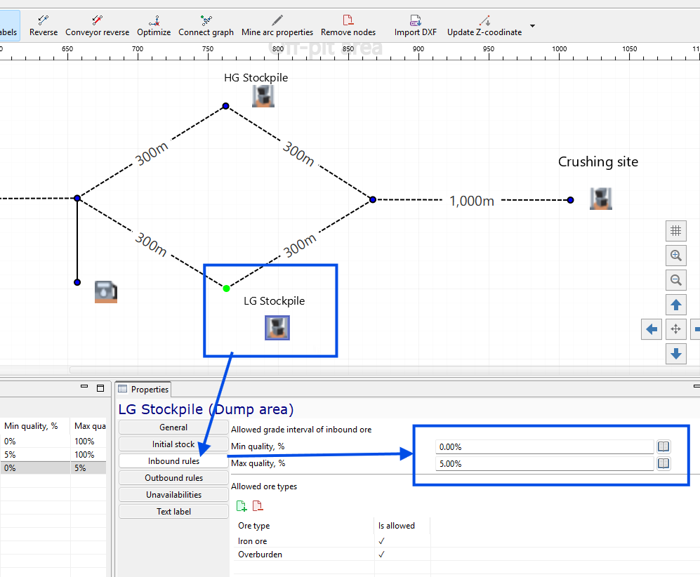
We add an LG Stockpile on the lower branch using the same approach. Its inbound rule accepts material from 0% to 5% quality, so low-grade ore can be routed separately from high-grade ore.

Download scenario

In this section, we will make the ore quality different across the four blocks. This will let us check whether the inbound quality rules route high-grade and low-grade material to the correct stockpiles.

After that, we will run the simulation and review the haulage volumes map and routes graph. We will also see why material stored in stockpiles is not yet counted as mined production in the current setup.

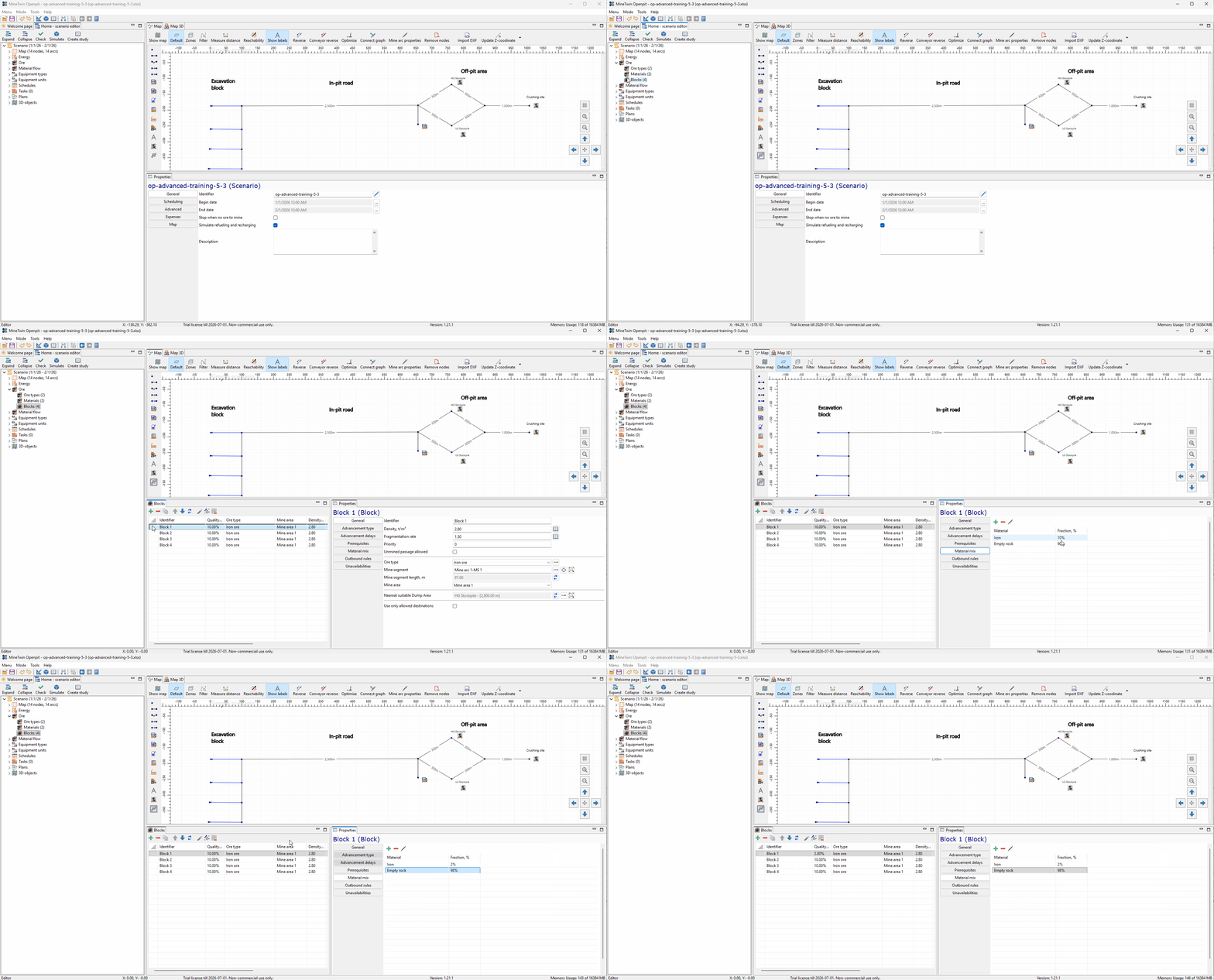
We set the ore fraction in Block 1 to 2%. This changes Block 1 into a low-grade block, so its material should be routed to the LG Stockpile.

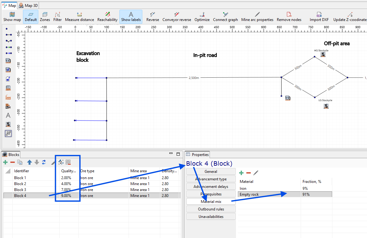
We set different ore qualities for the remaining blocks. The blocks now have 2%, 4%, 7%, and 9% quality, so the model contains both low-grade and high-grade material.

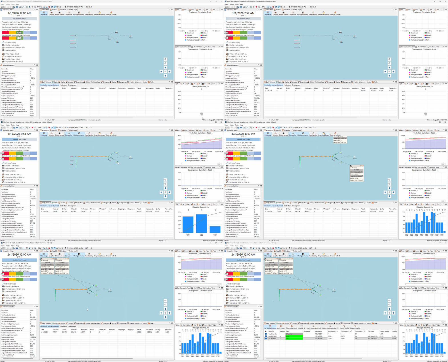
We run the simulation and review the haulage volumes map and stockpile table. The map shows high-grade blocks routed to the HG Stockpile and low-grade blocks routed to the LG Stockpile, while the stockpile table shows both stockpiles active with stored ore.

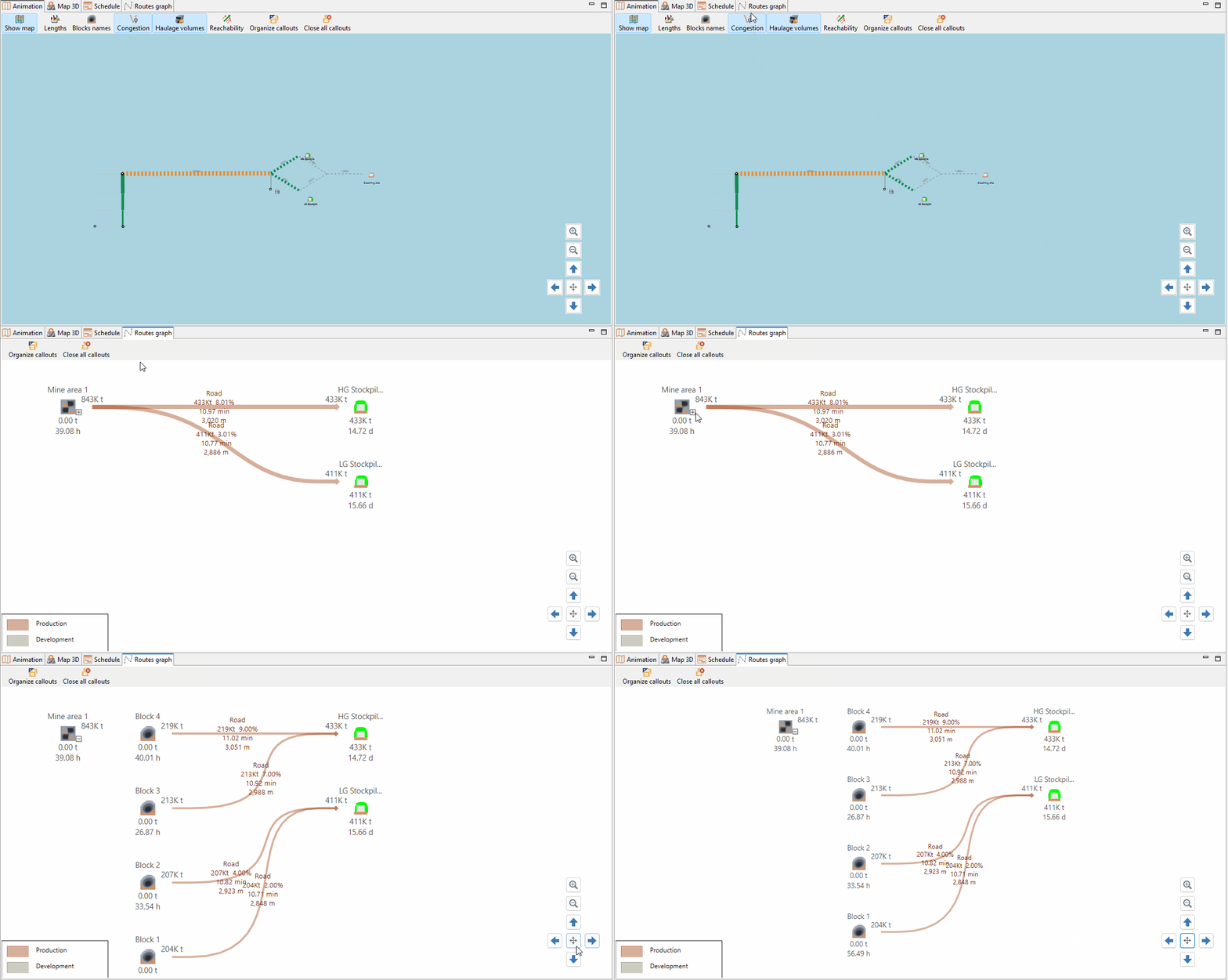
We review the routes graph to confirm that the stockpile grade limits are respected. Blocks with 7% and 9% quality are routed to the HG Stockpile, while blocks with 2% and 4% quality are routed to the LG Stockpile.

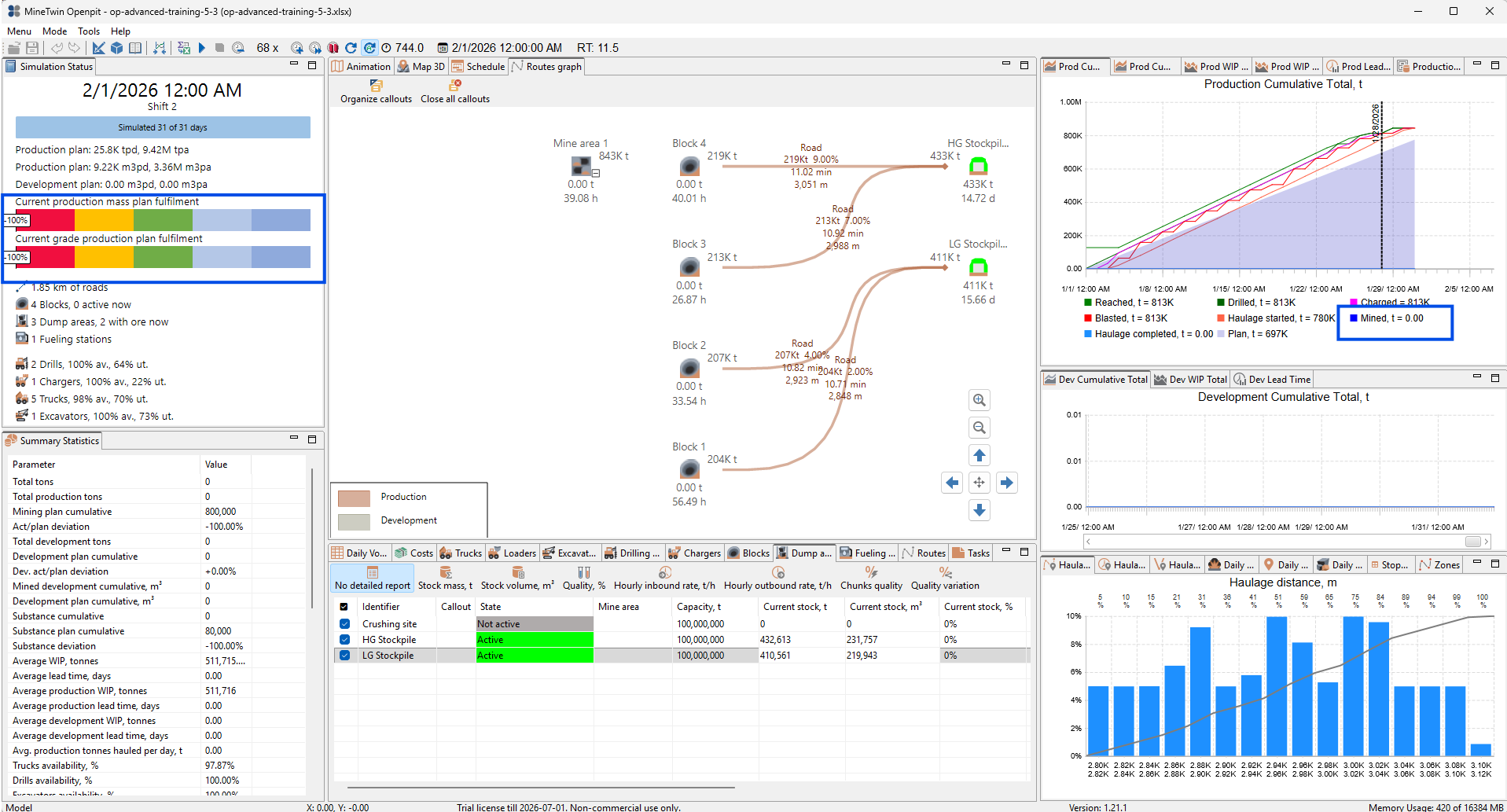
We note that production target fulfillment is now zero even though material has been hauled into stockpiles. This happens because, in the current setup, production is recognized only when material reaches the Crushing site mine area, not when it is stored in intermediate stockpiles.

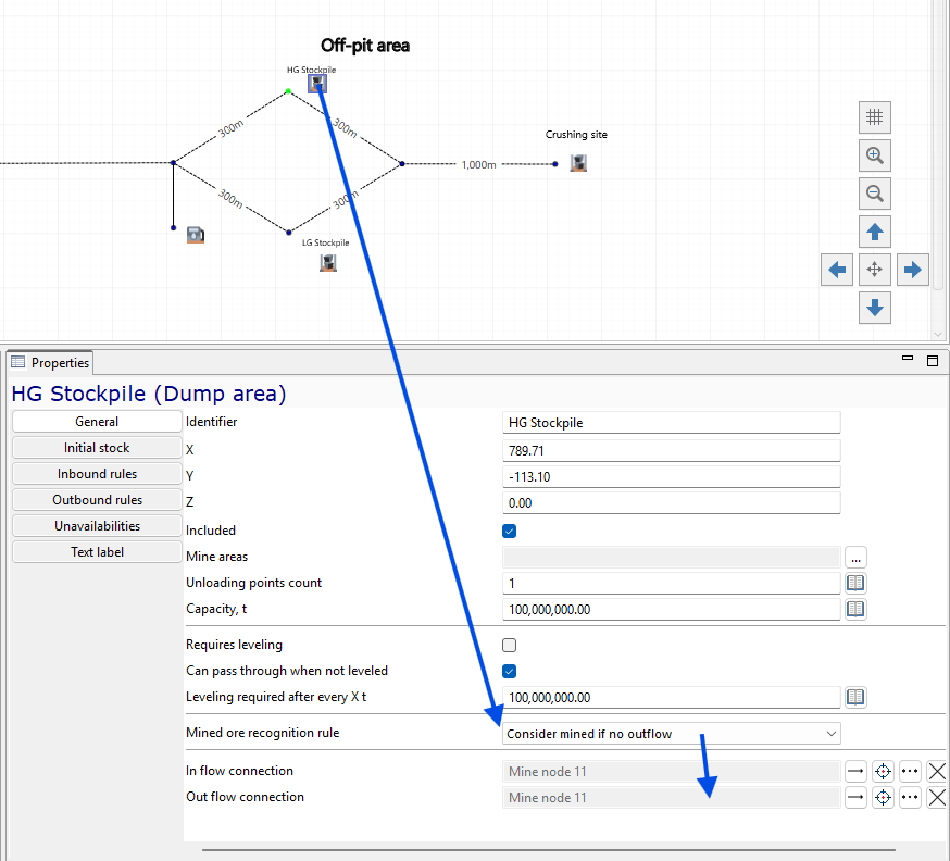
We review the stockpile mined ore recognition rule. The stockpiles use Consider mined if no outflow, but they already have outflow connections, so material stored there is treated as work in progress until the second leg of transportation is added.

Download scenario

In this section, we will add the equipment required to move ore from the stockpiles to the Crushing site. The first transportation leg has already moved material from blocks to stockpiles, but the second leg needs loaders to load material out of the stockpiles.

After adding the loader, we will run the simulation and check whether material reaches the Crushing site. We will also review the grade balance and adjust the target plan to match the blended material that arrives after the second leg.

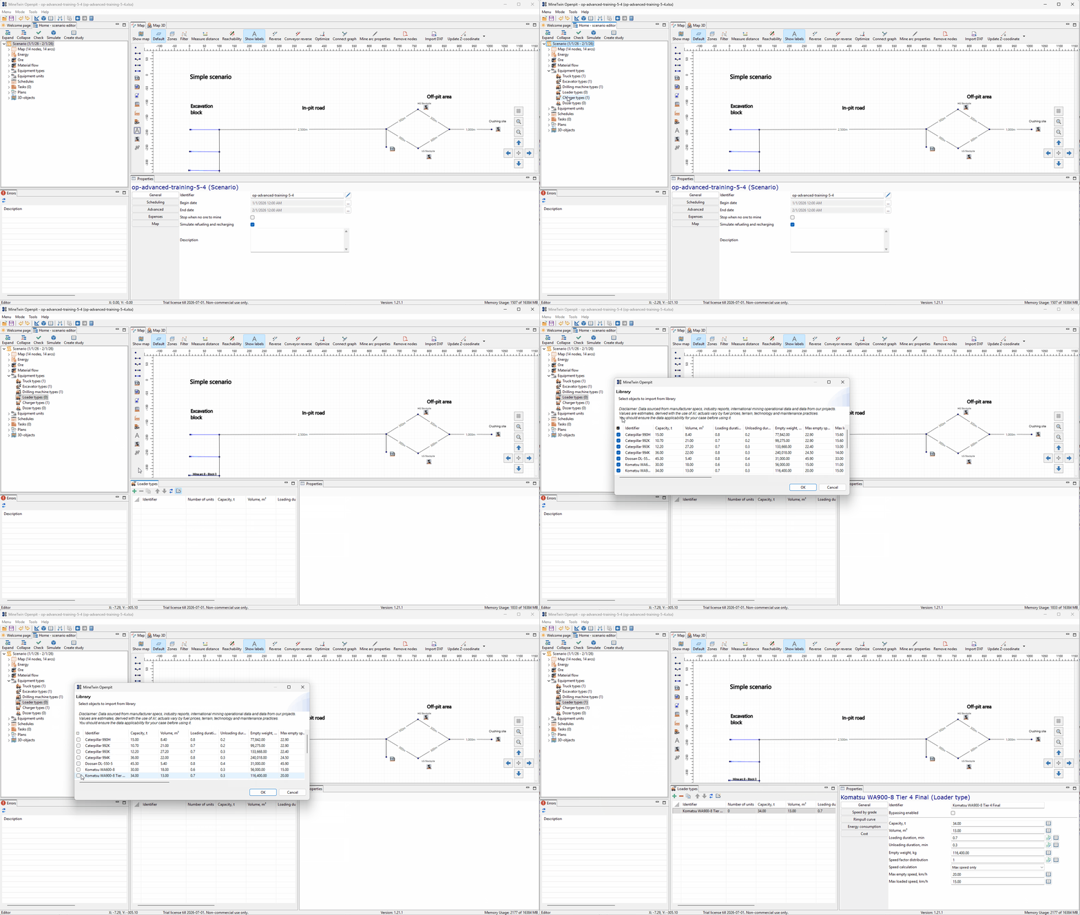
We add a loader type from the MineTwin library. In this example, we select the Komatsu WA900-8 loader type, and its loading, unloading, speed, and fuel-related parameters are populated from the library.

We check the imported loader type and correct the fueling rate value. The error panel shows that the fueling rate must be a positive number, so we update the value before creating a loader unit.

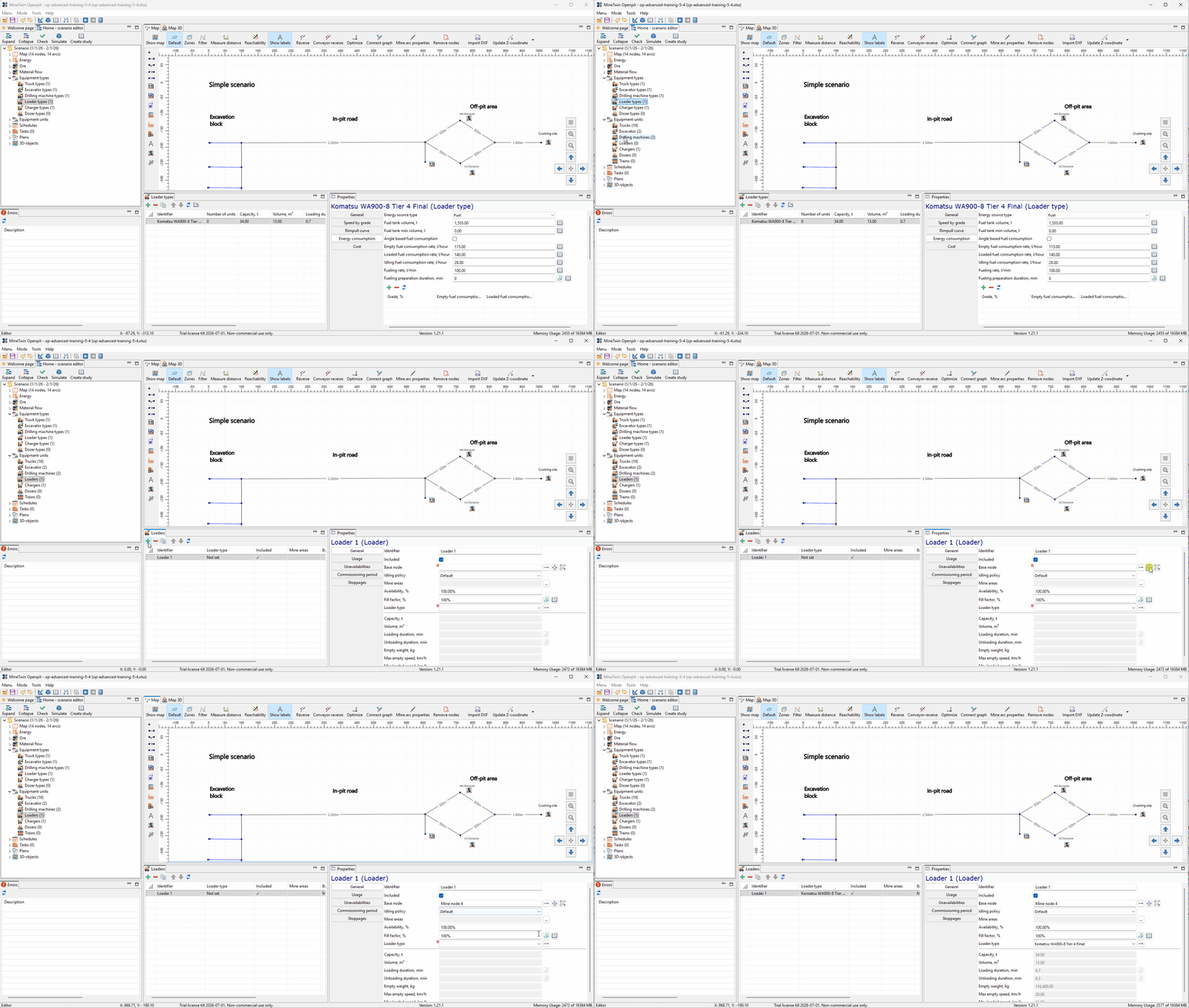
We add one loader unit and assign it to an off-pit base node. This gives MineTwin equipment that can load material out of the stockpiles for the second leg of transportation.

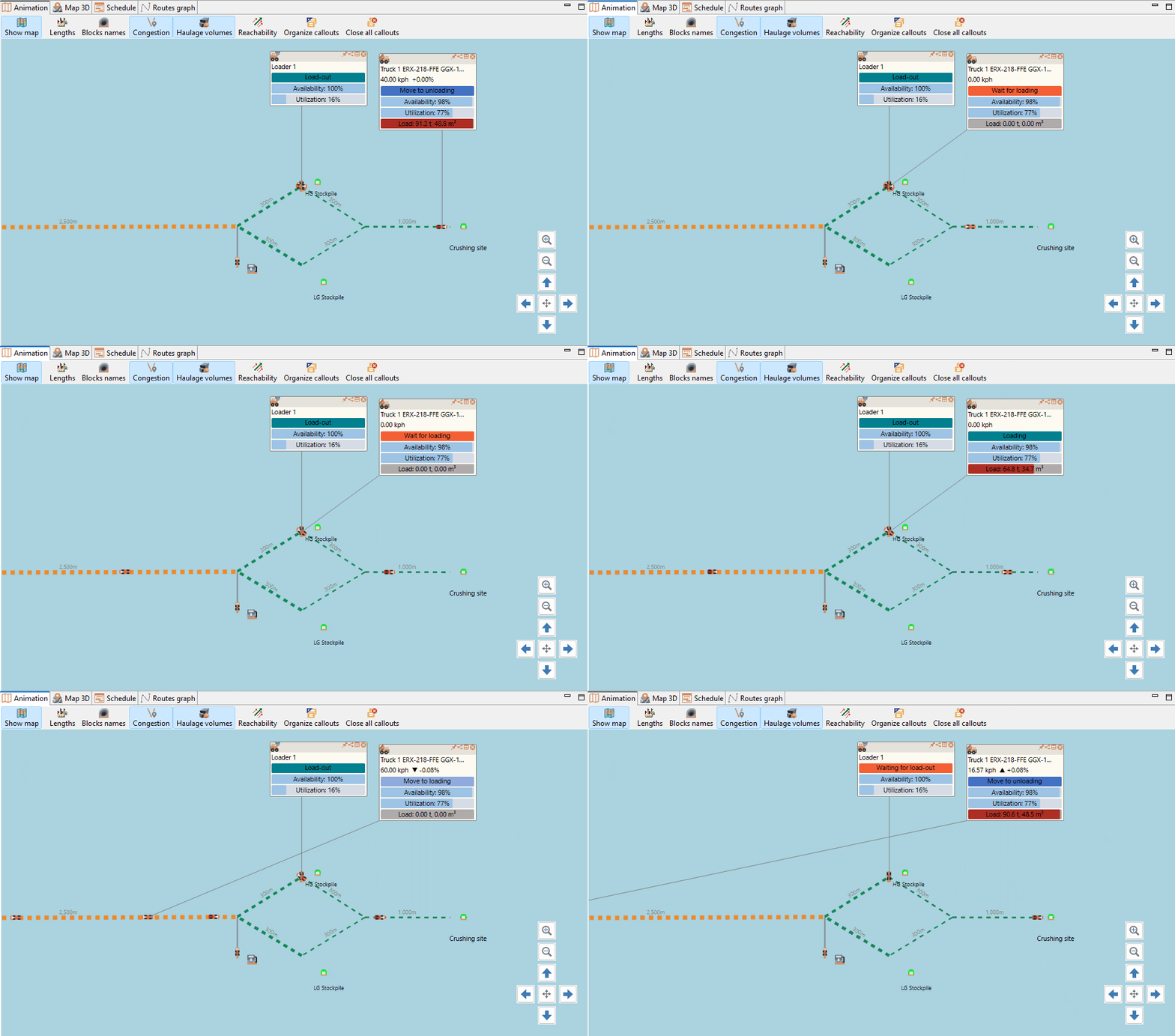
We run the simulation and review the animation. The second leg is now active: trucks move material from the stockpiles toward the Crushing site, and the loader works at the stockpile area to support load-out.

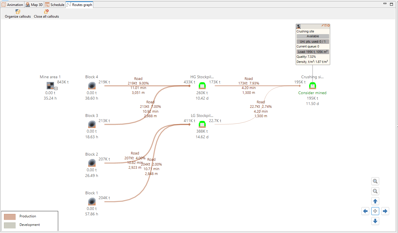
We review the routes graph and compare the material moved from the stockpiles to the Crushing site. Only part of the stockpiled material reaches the final destination, and the Crushing site quality is about 7.32%, which shows that the delivered blend does not match the previous 10% target quality.

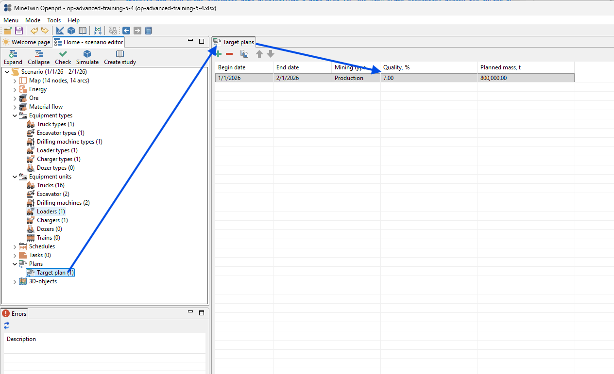
We adjust the target plan quality to 7%. This makes the production target more consistent with the blended ore quality that can be achieved after routing material through the high-grade and low-grade stockpiles.

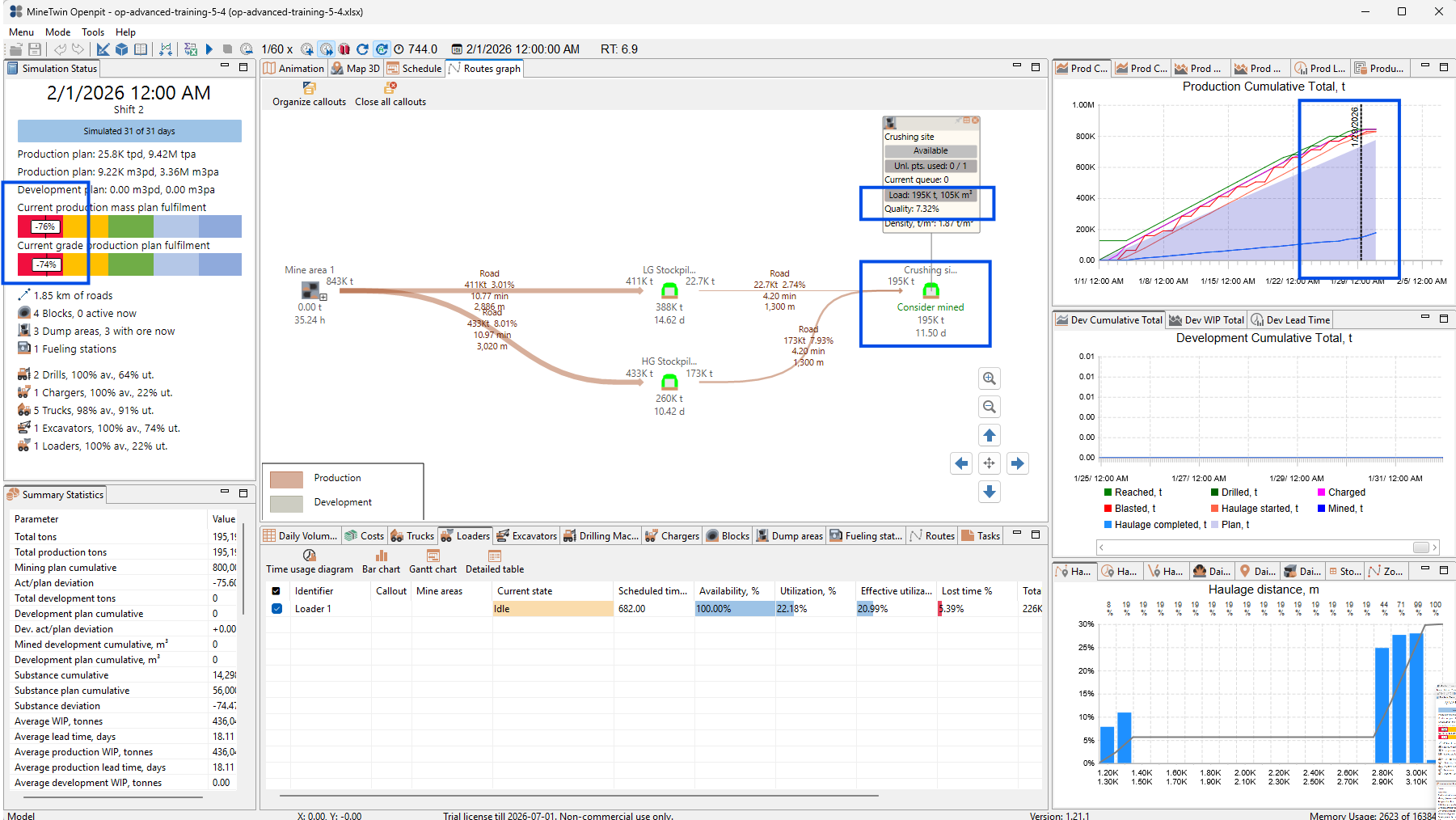
We run the simulation again after balancing the target quality. The scenario now recognizes production at the Crushing site, but the plan is still not fulfilled. The result shows that the current second-leg configuration does not have enough truck and loader capacity to move the required amount of material from the stockpiles to the Crushing site.

Download scenario

In this section, we will right-size the truck and loader fleet for the two-leg transportation setup. We will vary the number of trucks and loaders together, analyze which combinations reach the production target, and then choose the lowest-cost feasible configuration.

This study is interactive because the two resources constrain each other. Adding trucks alone may not help if loaders cannot load stockpiles fast enough, and adding loaders alone may not help if there are not enough trucks to move material to the Crushing site.

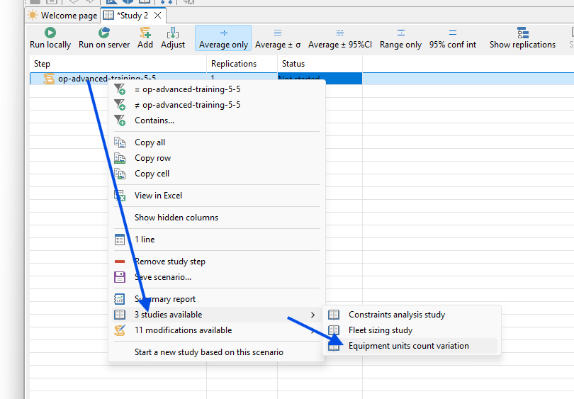
We create a variation study for the number of trucks. This will be the first study axis and will let MineTwin test several truck fleet sizes against the same scenario.

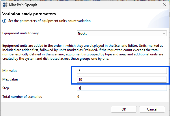
We set the truck count variation range from 5 to 10 with a step of 1. This creates six truck fleet options for the study.

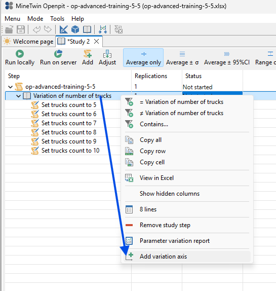
We add a second variation axis to the same study. This turns the study into a two-parameter sensitivity analysis where truck count and loader count are evaluated together.

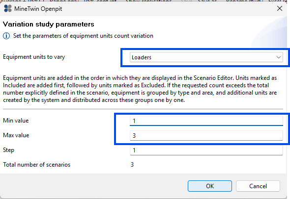
We configure the second axis as a loader count variation. The study will test 1 to 3 loaders with a step of 1, so each truck fleet size is combined with three loader fleet sizes.

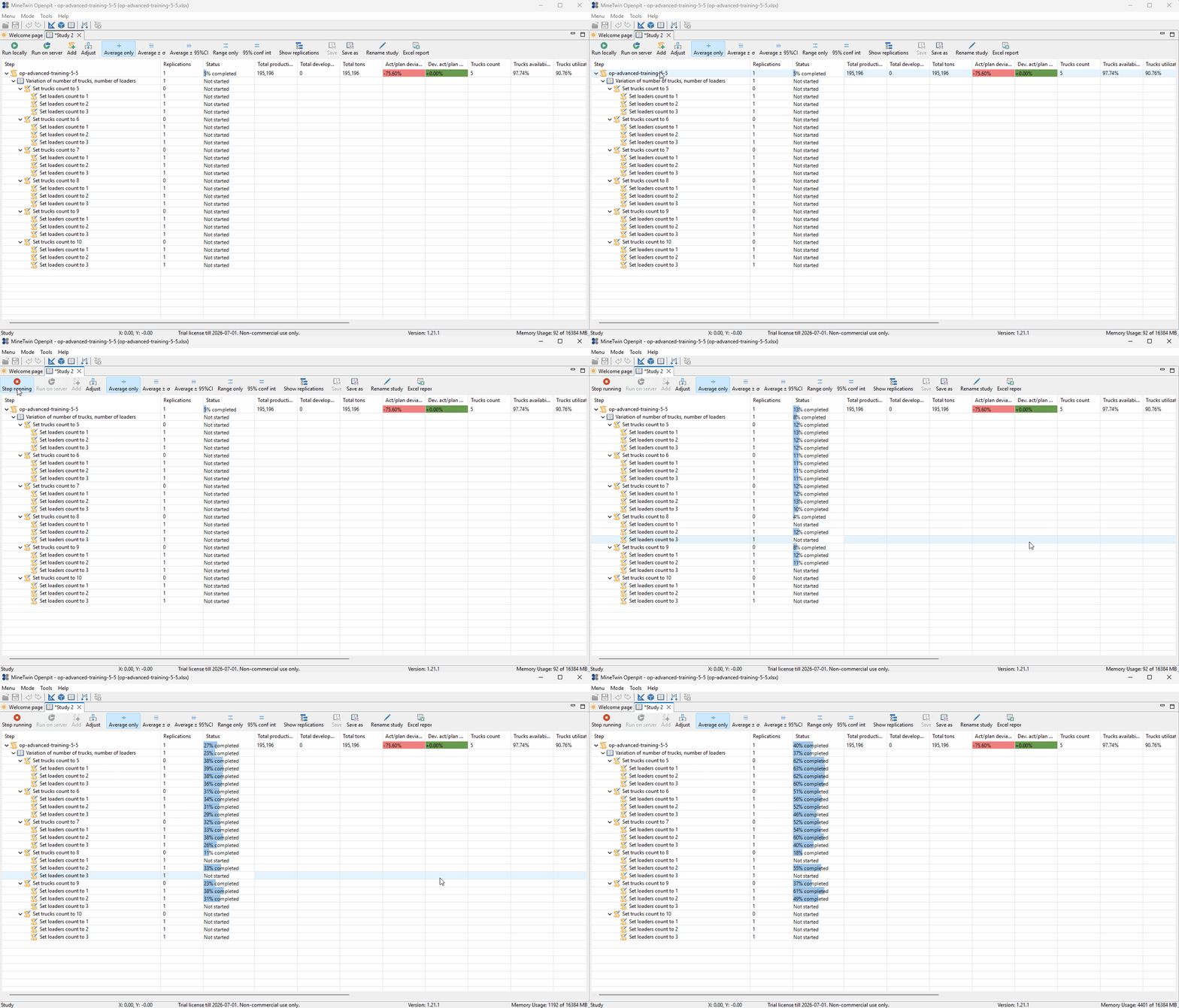
We run the initial study locally and wait for the scenarios to complete. At this stage, each truck-loader combination is calculated once, which is enough for a first screening of feasible configurations.

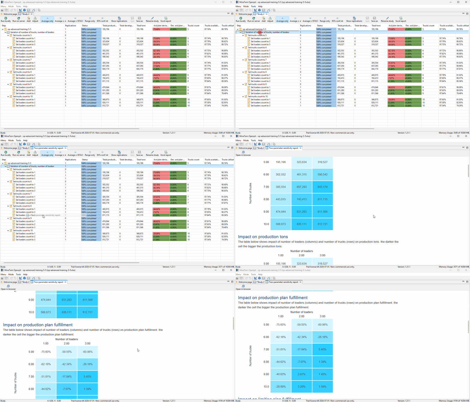
We open the two-parameter sensitivity report and review the production plan fulfillment heatmap. Rows represent truck counts, columns represent loader counts, and darker cells show better fulfillment of the production plan.

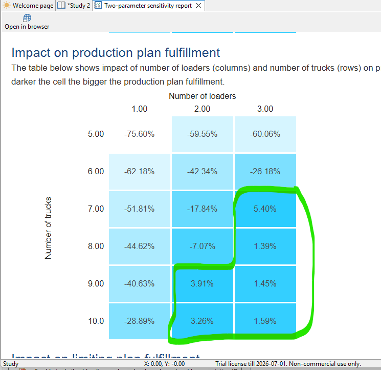
We identify the area of the heatmap where the production target is reached. The first run suggests that several combinations can fulfill the plan, including configurations with 2 or 3 loaders and higher truck counts.

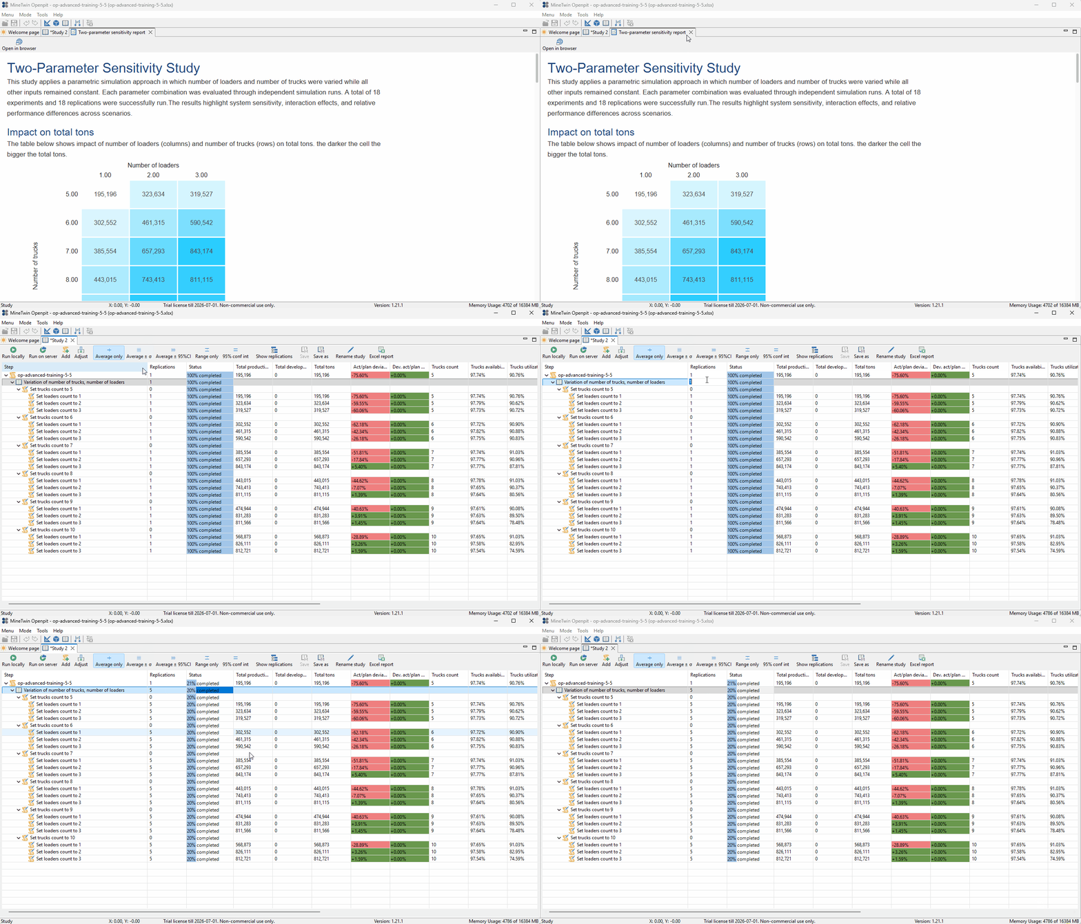
We increase the number of replications to 5 for the study. This gives more statistical confidence in the results and helps us avoid choosing a fleet configuration based on a single random run.

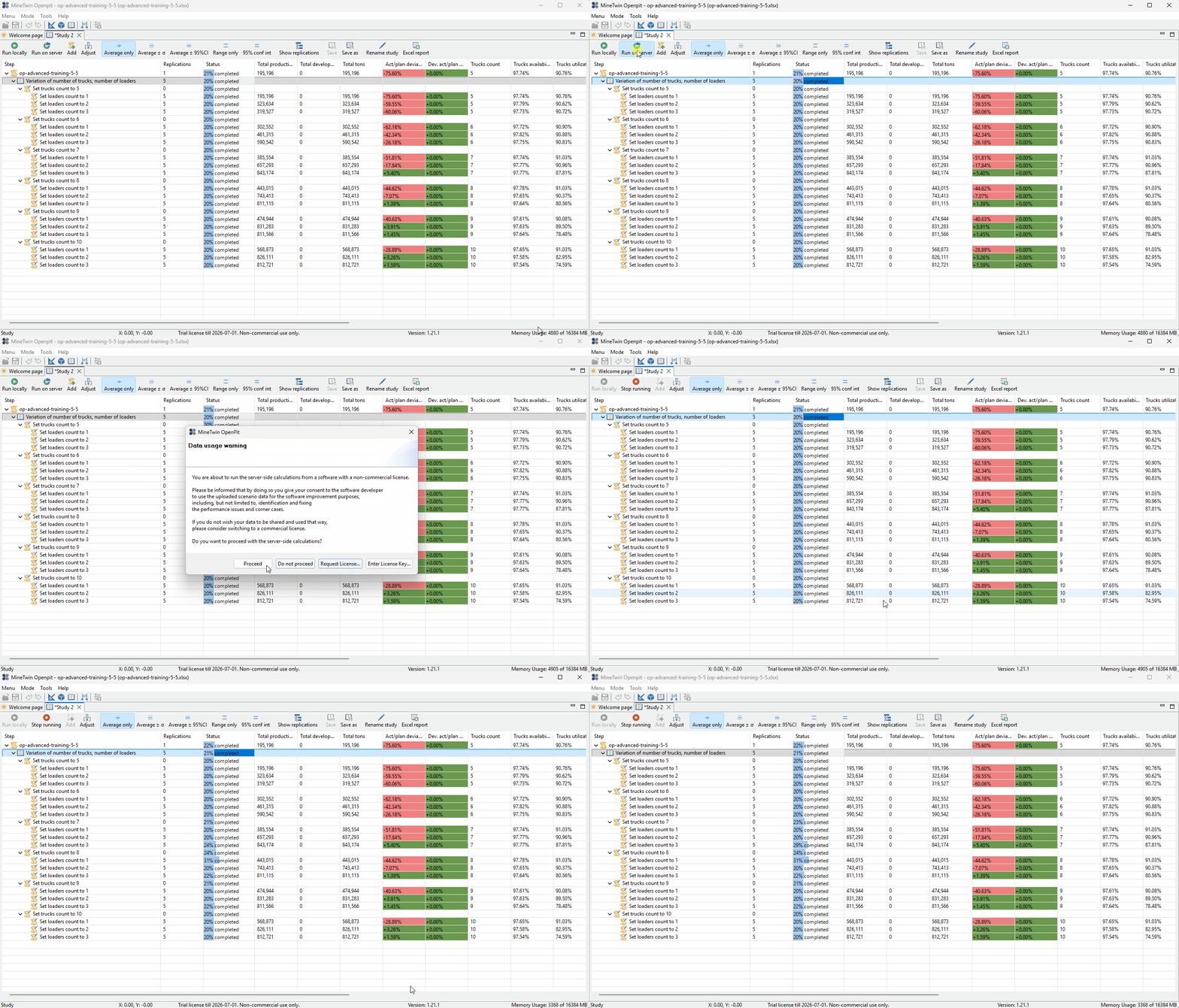
We run the additional replications on the server. This lets MineTwin calculate the larger batch of stochastic simulations without loading all computation onto the local application.

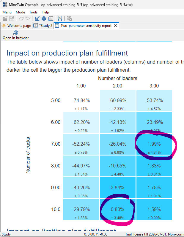
We review the updated heatmap and identify two critical configurations near the feasibility boundary: 7 trucks with 3 loaders, and 10 trucks with 2 loaders. Both are close to the target, so they need additional attention before we make the final fleet decision.

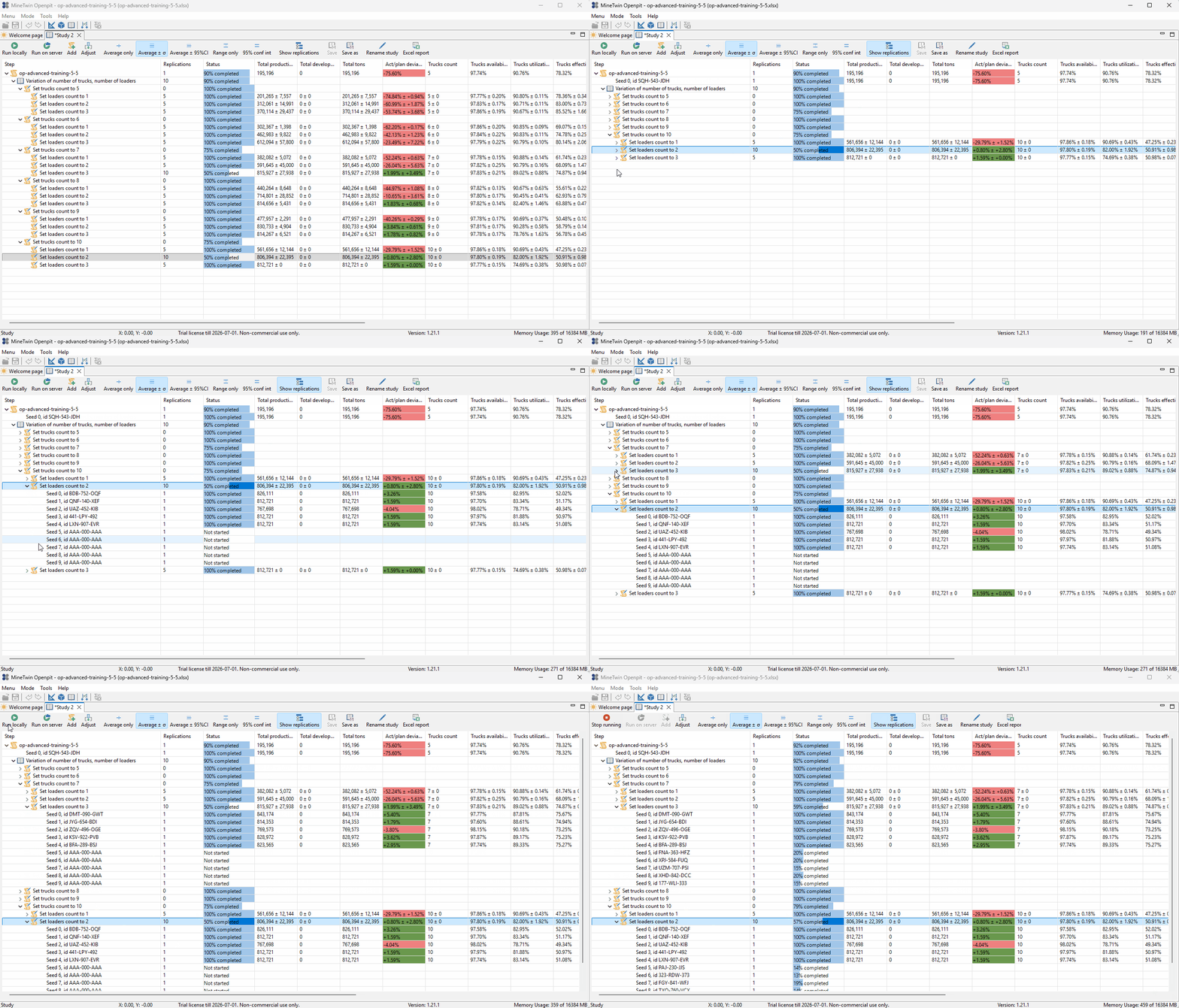
We show all replication results and run extra replications for the critical configurations. This helps confirm whether the observed target fulfillment is stable or only the result of random variation.

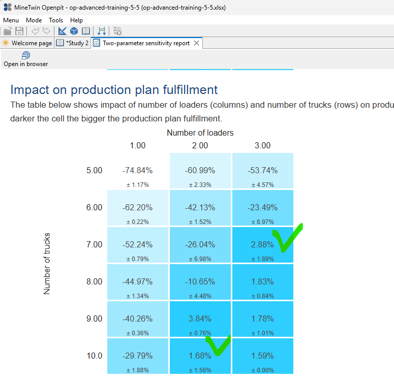
We review the updated report after the extra replications. The results confirm that 7 trucks with 3 loaders and 10 trucks with 2 loaders can both reach the production target under variability.

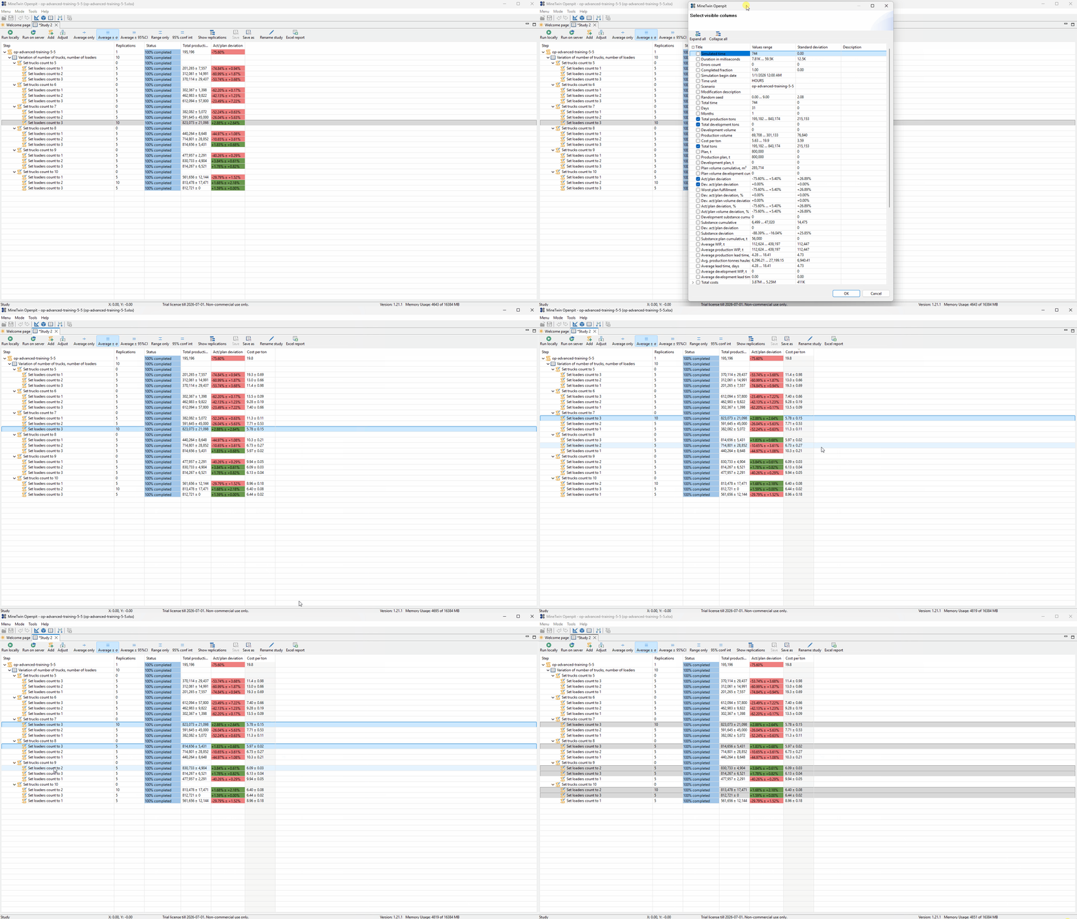
We add the Cost per ton column and compare the feasible configurations. The 7 trucks and 3 loaders configuration reaches the target with the lowest visible cost per ton, so it becomes the preferred scenario.

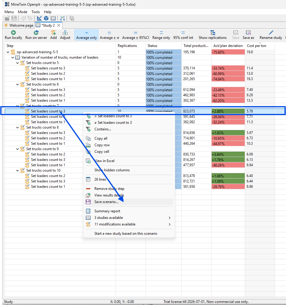
We save the best scenario based on cost per ton. This gives us a separate scenario file with the selected truck and loader fleet configuration.

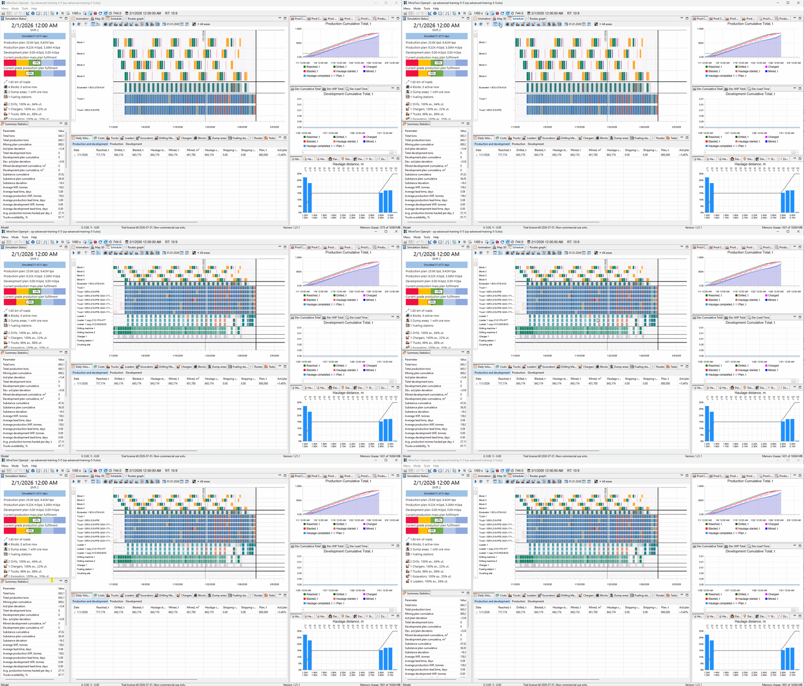
We run the saved scenario and review the simulation. The result shows that loaders are not fully utilized all the time because the second leg is constrained by cyclic interactions between stockpile availability, truck arrivals, loading, hauling, and unloading at the Crushing site.

Download scenario