Make the simulation more realistic and run first simulation studies
1. Review the main indicators of the first simulation
In this section, we will review the main outputs from the first working simulation. We will look at the simulation status, cumulative production chart, routes graph, and truck time usage diagram to understand why the initial scenario does not reach the production target.
This review gives us a baseline before we start changing the scenario. We will use these indicators to identify the current bottleneck and prepare for the first simulation studies.
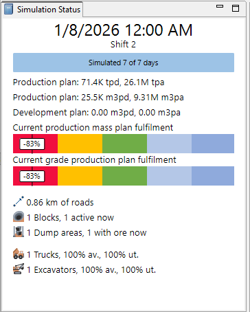
We start with the Simulation Status panel. It shows that the model has simulated the full 7-day period, from January 1 to January 8, 2026, with one active block, one dump area containing ore, one truck, and one excavator. The production mass and grade fulfillment indicators are both at -83%, which means the scenario is significantly behind the target.
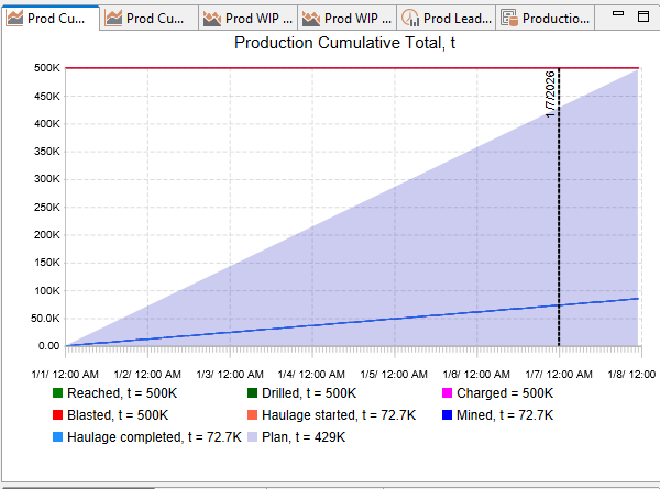
Next, we review the Production Cumulative Total chart. The planned production reaches 500,000 t by the end of the period, while the actual mined and haulage completed values reach only about 72.7K t. This confirms that the first configuration is valid and running, but the available fleet is not sufficient to meet the plan.
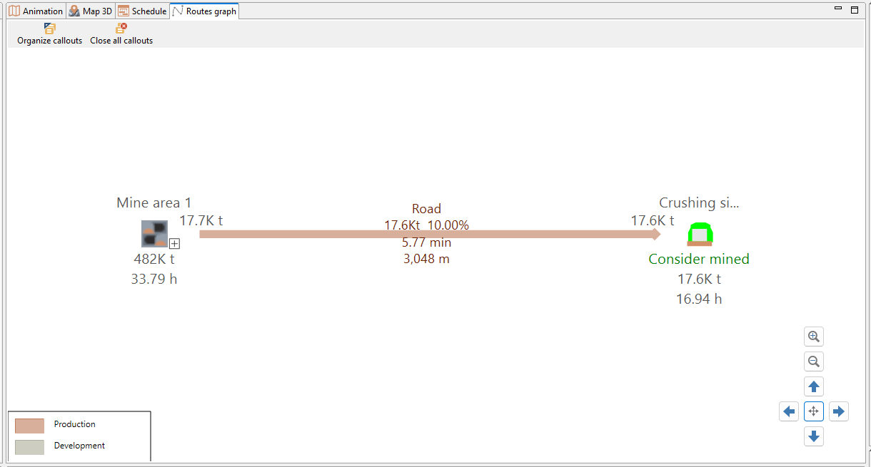
We then open the Routes graph to see how material moves through the model. The graph shows production flow from Mine area 1 to the Crushing site, which is the dump area we created earlier. It also shows the road segment between them, including hauled tonnage, travel time, and haulage distance, so we can connect the production result with the physical haulage path.
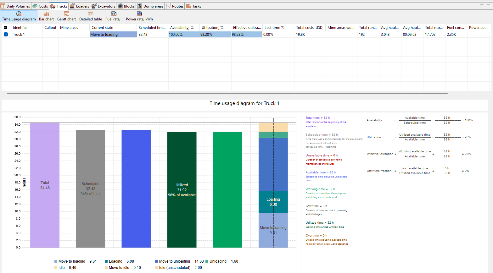
Finally, we review the truck time usage diagram for Truck 1. The table shows 100% availability and 98% utilization, and the diagram breaks the scheduled time into operating states such as moving to loading, loading, moving to unloading, unloading, and idle time. This helps us see that the truck is almost constantly used, which suggests that increasing fleet capacity may be a reasonable next study.
2. Run fleet sizing study
In this section, we will run the first simulation study to evaluate how the fleet configuration affects production. We will use a fleet sizing study to compare the baseline scenario with several equipment adjustment options and identify a better configuration.
The goal is not only to increase production, but also to understand which equipment is limiting the current scenario. We will review the study table, open the summary report, and save the best scenario configuration for the next step of the training.
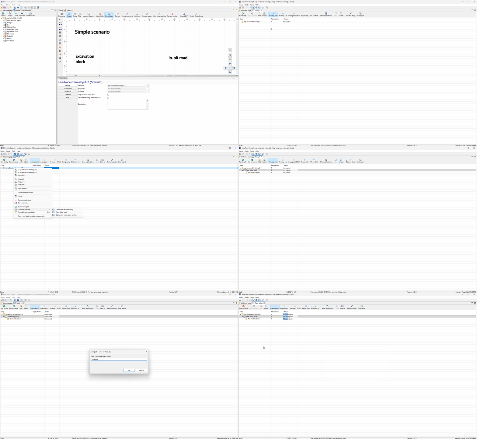
We switch the model to Study mode, select the Fleet sizing study type, and rename the study tab to Fleet sizing. After that, we run the study locally. The study starts from the baseline case with no modifications, then evaluates equipment adjustment options and reports the completion status and key indicators for each run.
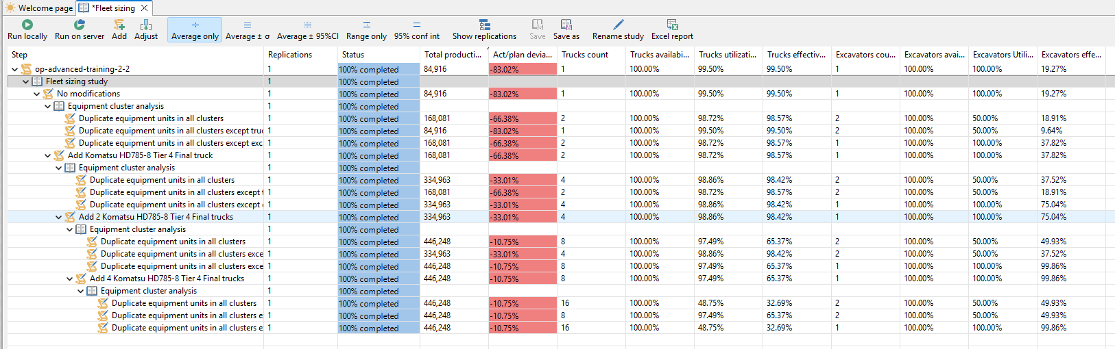
We review the completed fleet sizing study results. Fleet sizing searches for the minimum mobile equipment configuration required to achieve the target production and development plans. The study first calculates the No Modifications baseline and identifies equipment clusters, where each cluster is a group of equipment with the same class, type, and assigned operating area. MineTwin then tests adding equipment to these clusters, compares the effect of each change, and repeats the process until the plan can be fulfilled. After that, it tries removing the least utilized equipment units to reduce the fleet while keeping the plan achievable. The process is shown as a hierarchical table with branching study steps, generated modifications, and key indicators. In this run, the best visible result reaches 446,248 t with 8 trucks and 1 excavator, reducing the plan deviation from -83.02% to -10.75%, but still not fully reaching the target.
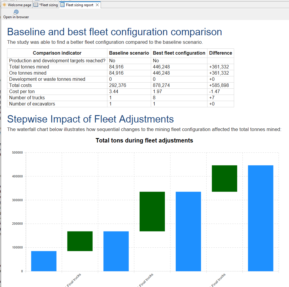
Next, we open the fleet sizing report. The report compares the baseline scenario with the best fleet configuration and shows that production increases from 84,916 t to 446,248 t. It also shows that the cost per ton decreases from 3.44 to 1.97, while the number of trucks increases from 1 to 8 and the number of excavators remains 1.
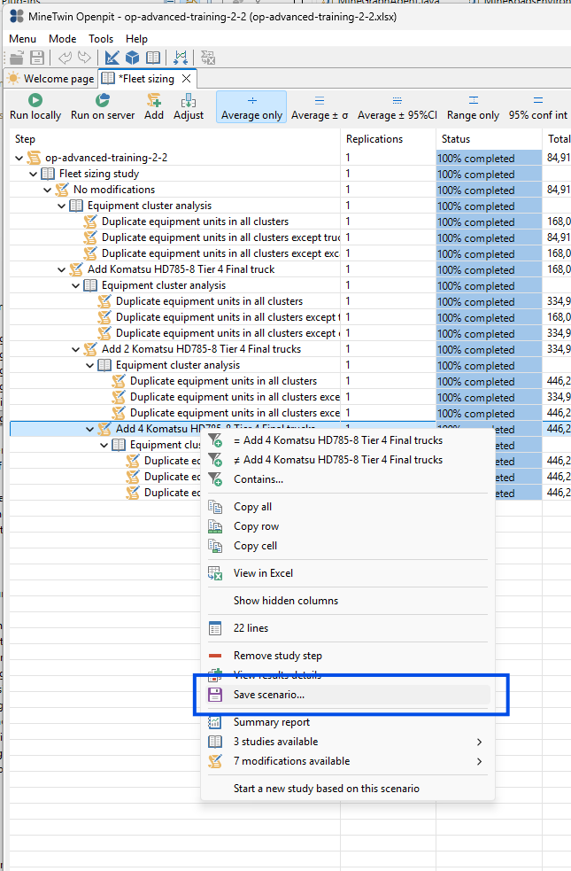
Finally, we save the selected fleet sizing result as a scenario. This creates a new scenario version based on the improved fleet configuration, so we can continue the training from the best study result instead of manually recreating the equipment changes.
3. Add another block with ore and rerun fleet sizing study
In this section, we will add a second ore block to the scenario and rerun the fleet sizing study. We will use this step to show how the recommended fleet changes when the mine has more than one active production source.
The previous fleet sizing result improved production, but it still did not fully reach the target. By adding another block, we give the model an additional mining front and allow MineTwin to evaluate whether extra loading capacity can improve the result.
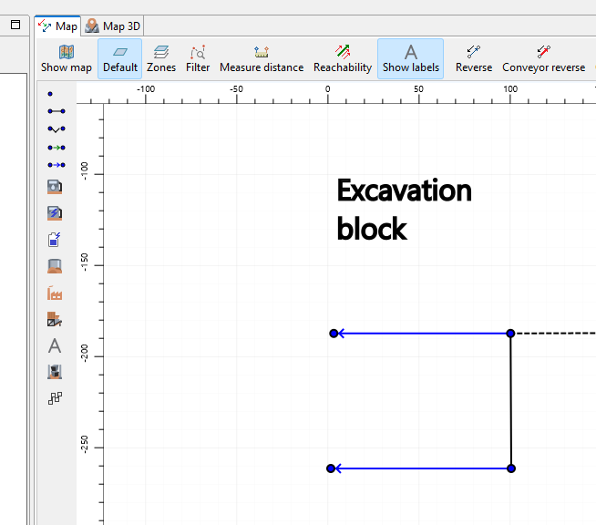
We add another block with ore on a second mine segment connected to the same road network. This creates an additional production source in the scenario, so the simulation can potentially use more loading equipment in parallel.
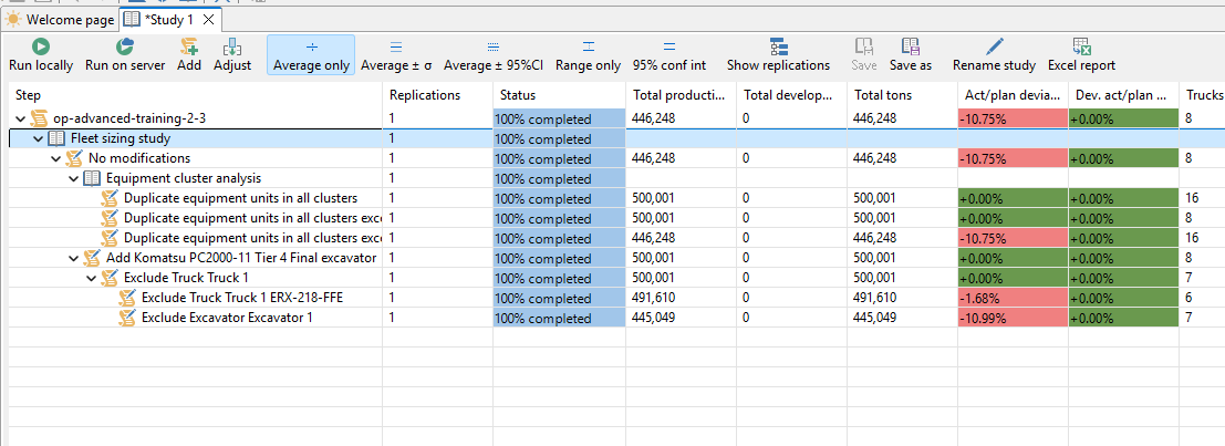
We rerun the fleet sizing study from the updated scenario. The study table shows that MineTwin starts from the previous improved configuration, then evaluates additional fleet changes for the new two-block layout. In this run, the study finds a configuration that can reach the 500,000 t production target by adding another Komatsu PC2000-11 excavator.
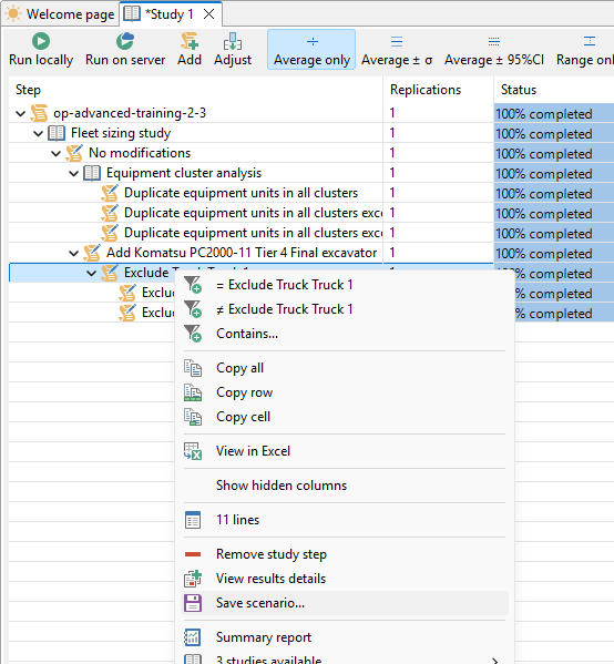
We save the selected fleet sizing result as a new scenario. This lets us continue from the configuration found by the study, where the model has additional loading capacity for the two-block setup.
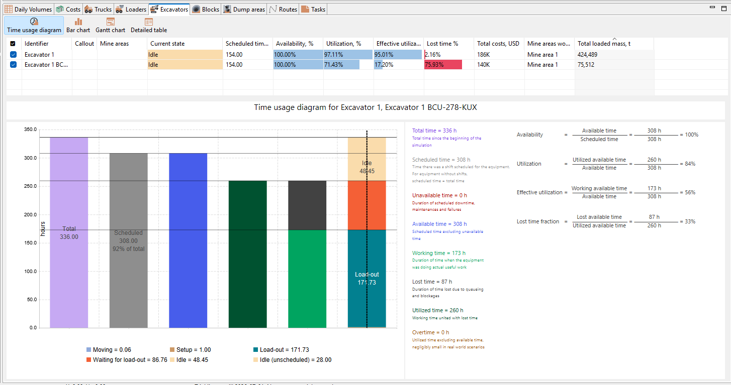
We review the simulation result with two excavators. The excavator table shows that the first excavator carries most of the loading work, while the second excavator contributes additional loaded mass but also has significant lost time. This indicates that the current equipment set is underutilized after the target is reached, so we can increase the production plan to make the next study more meaningful.
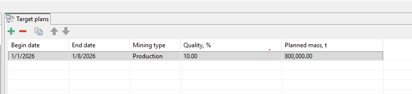
Finally, we increase the production target plan to 800,000 t for the same period. This creates a more demanding scenario that better uses the available loading capacity and prepares the model for the next study, where we will analyze how changing the number of trucks affects production.
4. Run trucks count variation study and analyze the results
In this section, we will move from automatic fleet sizing to a controlled parameter variation study. We will vary only the number of trucks and compare how this input affects production, plan fulfillment, utilization, and costs.
This study helps us understand the response curve of the model. Instead of asking MineTwin to choose the fleet automatically, we define the truck count range ourselves and analyze the resulting trade-offs.
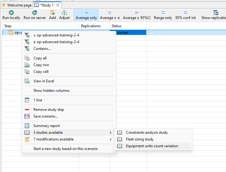
We start a new study based on the current scenario and select Equipment units count variation. This study type lets us vary the number of selected equipment units while keeping the rest of the scenario structure unchanged.
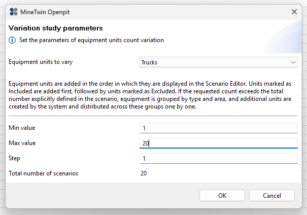
We configure the variation study to change the number of trucks from 1 to 20 with a step of 1. This creates 20 scenarios, allowing us to compare production and utilization across a wide range of truck fleet sizes.
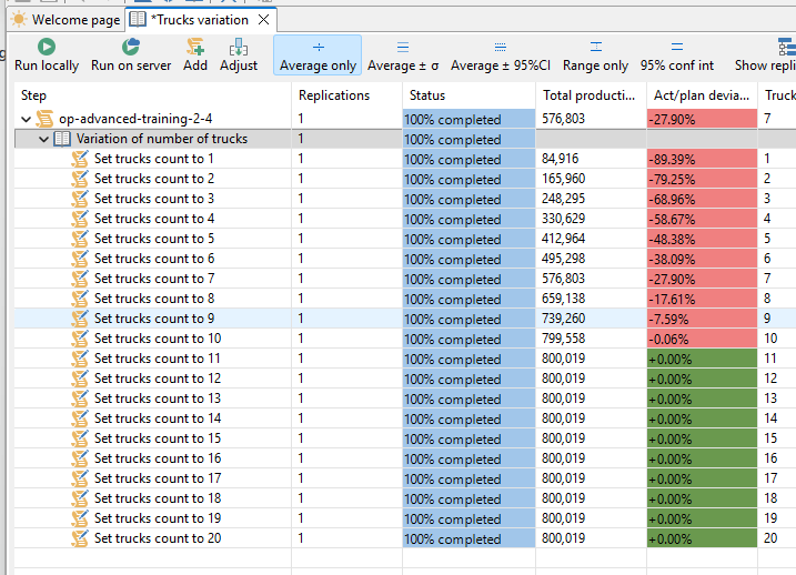
We review the completed trucks variation results. The table shows that production increases as the truck count grows, and the 800,000 t target is reached from 11 trucks onward. After that point, adding more trucks does not increase production, while truck utilization and effective utilization continue to decrease.
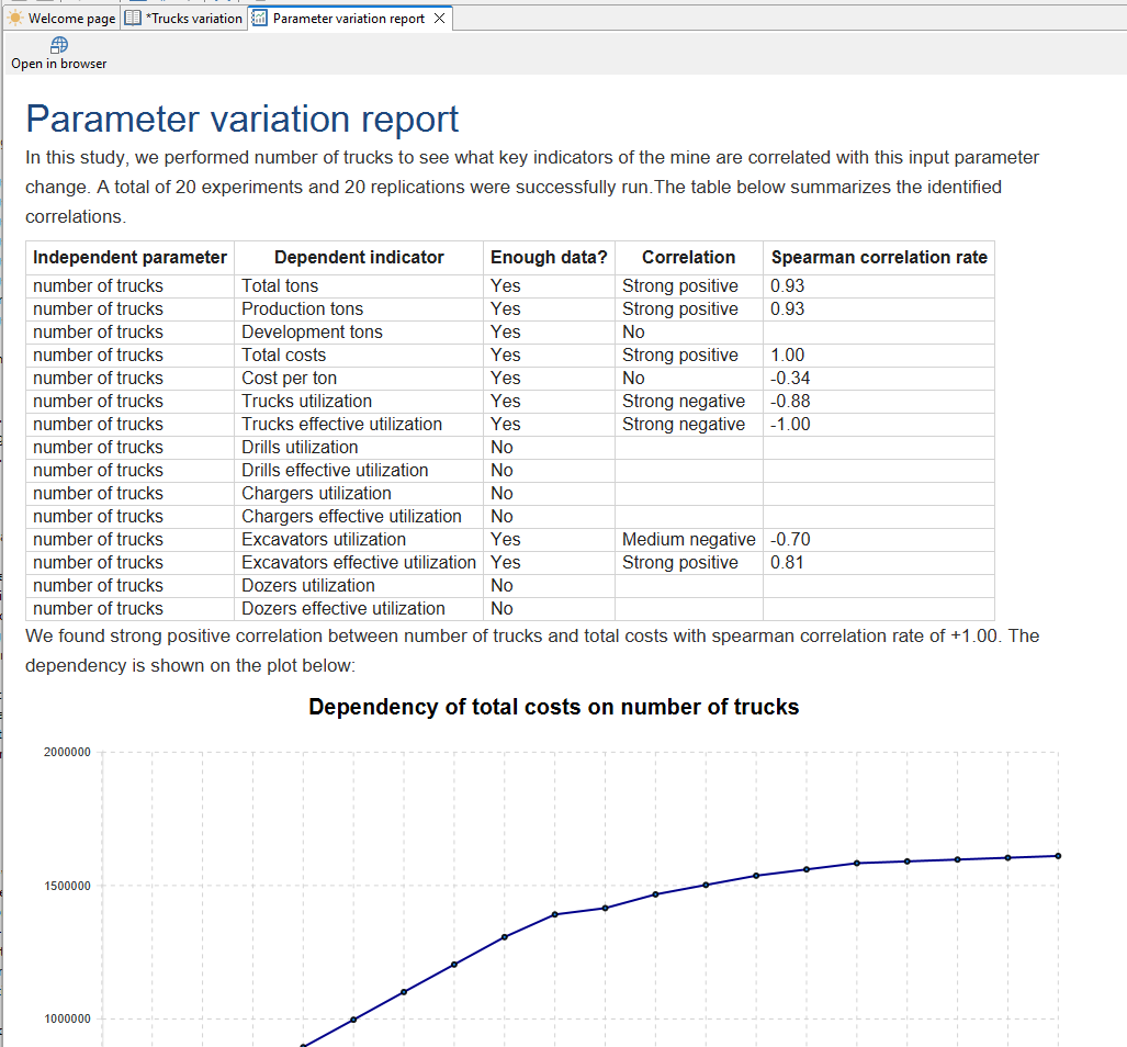
Next, we open the parameter variation report. The report summarizes correlations between the number of trucks and key indicators. It shows strong positive correlation with total tons, production tons, and total costs, and strong negative correlation with truck utilization and truck effective utilization.
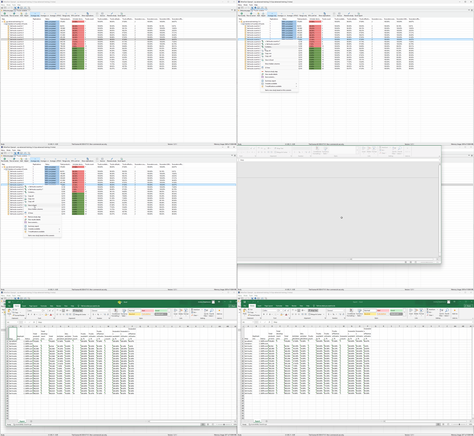
We export the study table to Excel for external review. The exported table includes the study steps, truck counts, production indicators, plan deviation, equipment counts, and utilization metrics, making it easier to inspect or share the results outside MineTwin.
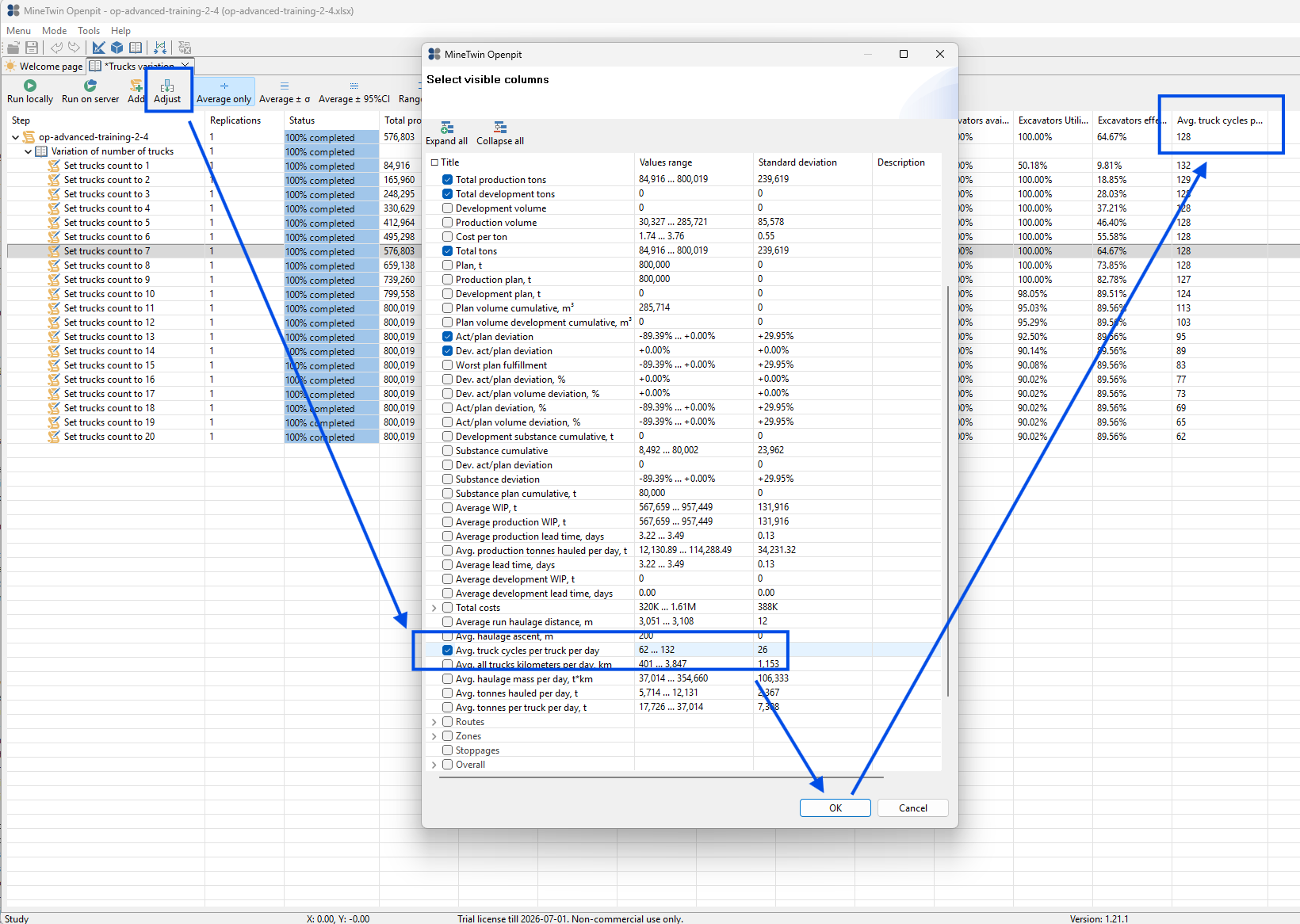
We adjust the visible columns in the study table and add Avg. truck cycles per truck per day. This indicator helps us compare how intensively each truck is used as the fleet size increases.
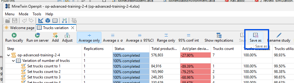
Finally, we save the completed study to a file. This preserves the variation results so they can be reopened later or shared together with the training materials.
5. Add real-world variability and use rimpull curves for trucks
In this section, we will make the model more realistic by adding variability and improving truck speed calculation. We will replace part of the deterministic setup with stochastic behavior, use rimpull curves for truck movement, and rerun the truck count variation study with replications.
This lets us move from a single deterministic result to a range of possible outcomes. We will then use confidence intervals and distributions to choose a more robust truck fleet configuration.
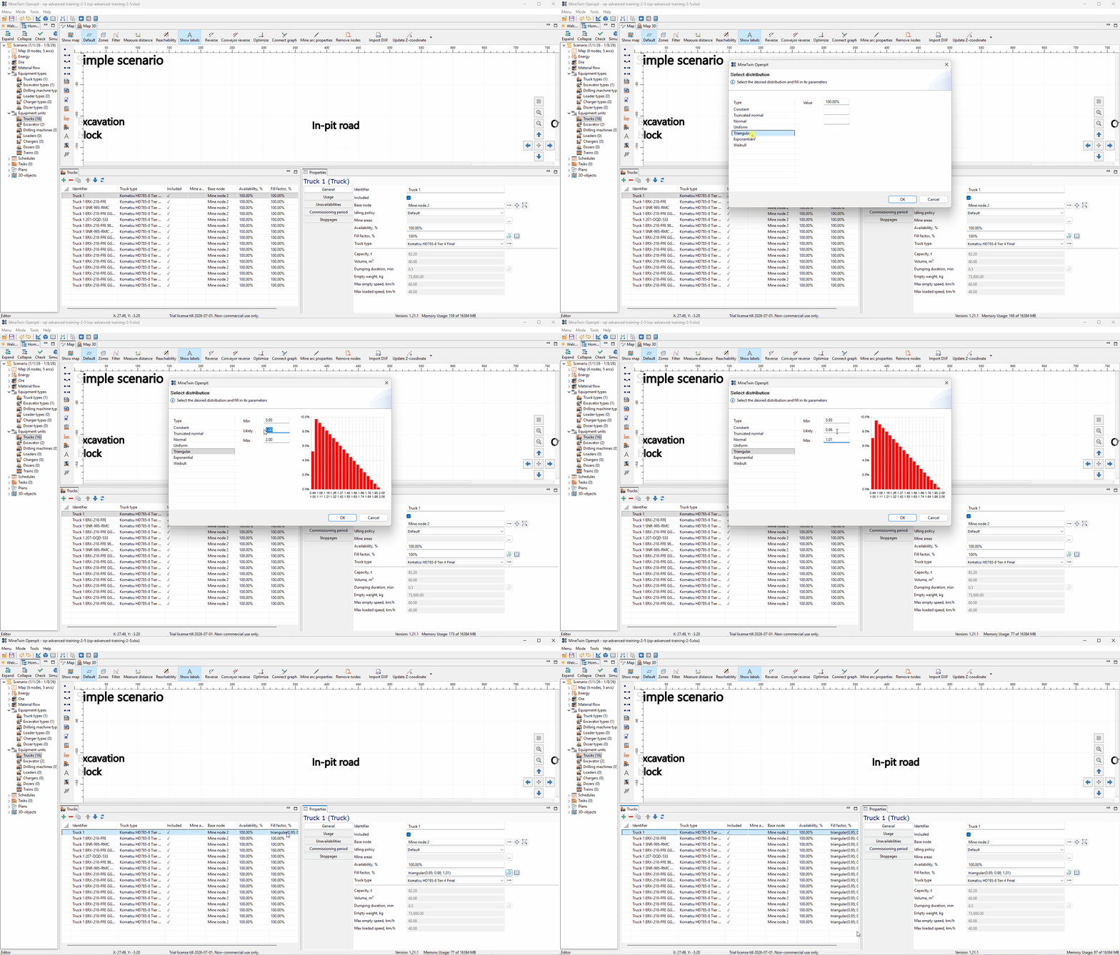
We start by changing the truck fill factor from a fixed value to a variable input. We set a triangular distribution with minimum 0.95, likely value 0.98, and maximum 1.01, and apply it to the truck units. This makes each truck load less perfectly predictable and reflects that real truck payloads vary from cycle to cycle.
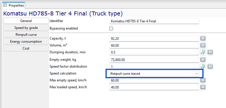
Next, we change the truck speed calculation method to Rimpull curve based. With this option, MineTwin calculates truck speed using the truck weight, road characteristics, gradient, rolling resistance, and rimpull curve data instead of relying only on fixed maximum loaded and empty speeds.
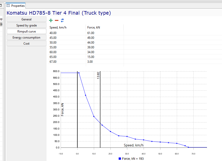
We review the rimpull curve for the Komatsu HD785-8 truck type. The curve describes the relationship between truck speed and available tractive effort, which MineTwin uses when calculating realistic movement speed on haul roads.
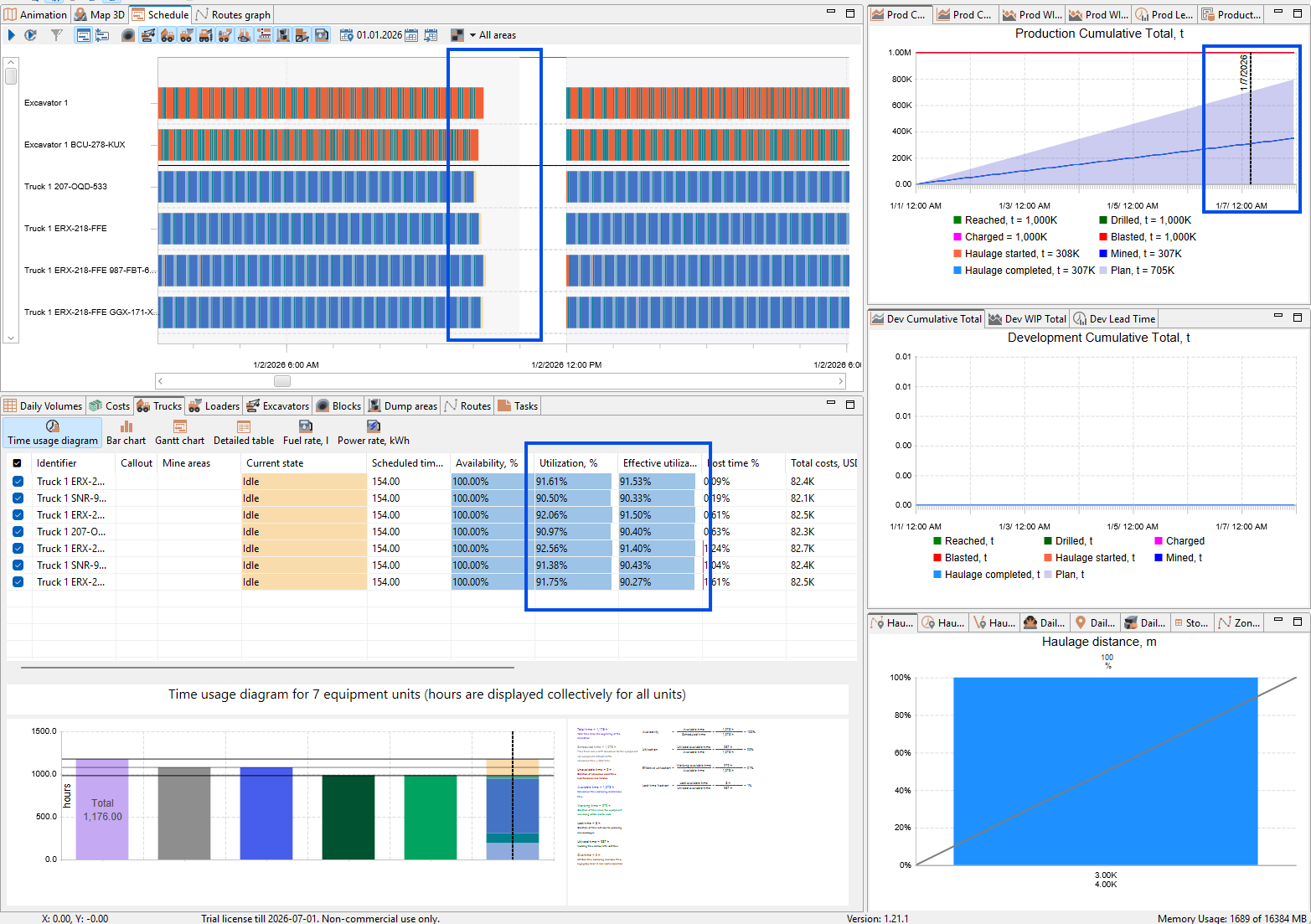
We run and review the scenario after adding variability and rimpull-based speed calculation. At this point, truck availability is 100%, but truck utilization remains around 91-93%, even though the trucks are expected to be busy almost continuously. This happens because only optimization-based planning is enabled, and it keeps some reserve for queues, waiting time, and operational variability.
This result prepares the next step: we will also enable dynamic planning. Dynamic planning will fill the remaining truck capacity during the shift and raise truck utilization closer to 99%.
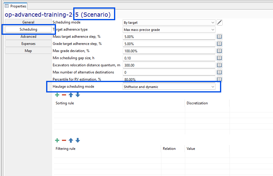
We change the haulage scheduling mode to Shiftwise and dynamic. This adds dynamic dispatching on top of the optimization-based plan, so truck assignments can be adjusted during the shift when additional hauling capacity is available.
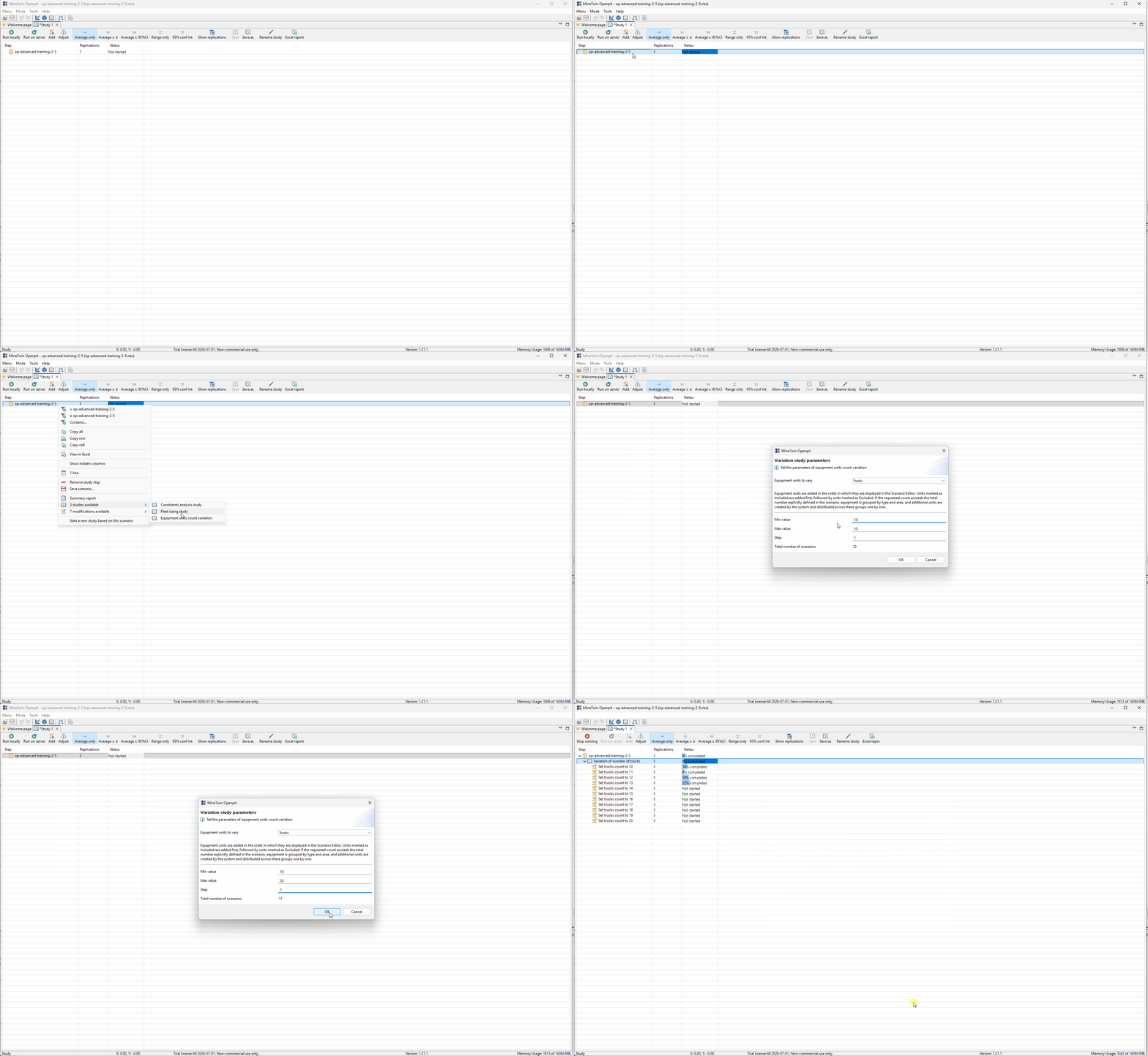
We rerun the trucks count variation study with three replications for each truck count. The study now evaluates truck counts from 10 to 20, and each replication uses a different random seed so the results reflect variability rather than a single deterministic run.
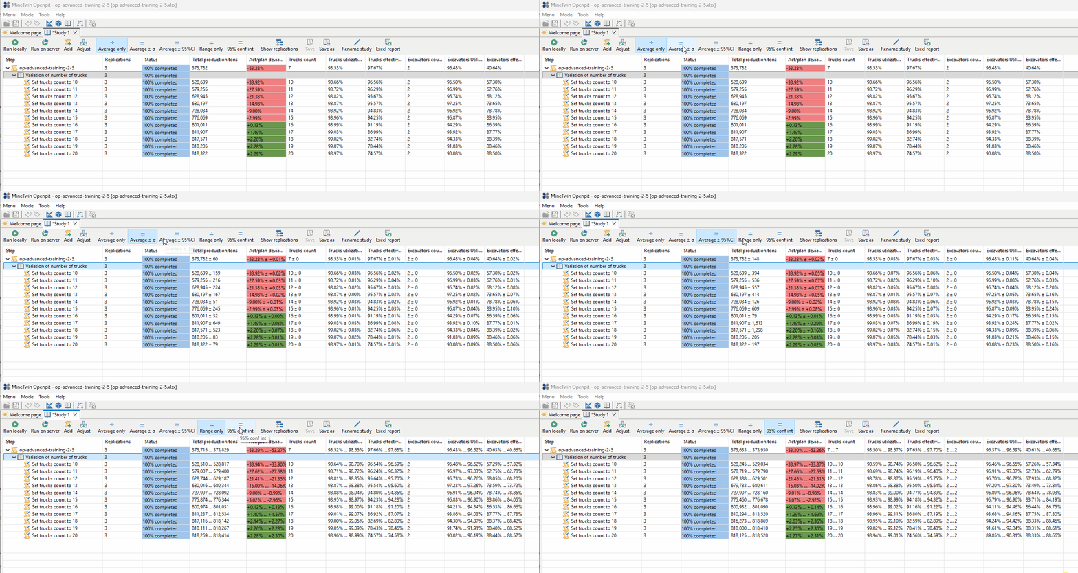
We switch the study result view from single average values to statistical summaries. MineTwin can show result ranges, averages with standard deviation, and 95% confidence intervals, which helps us compare alternatives under uncertainty.
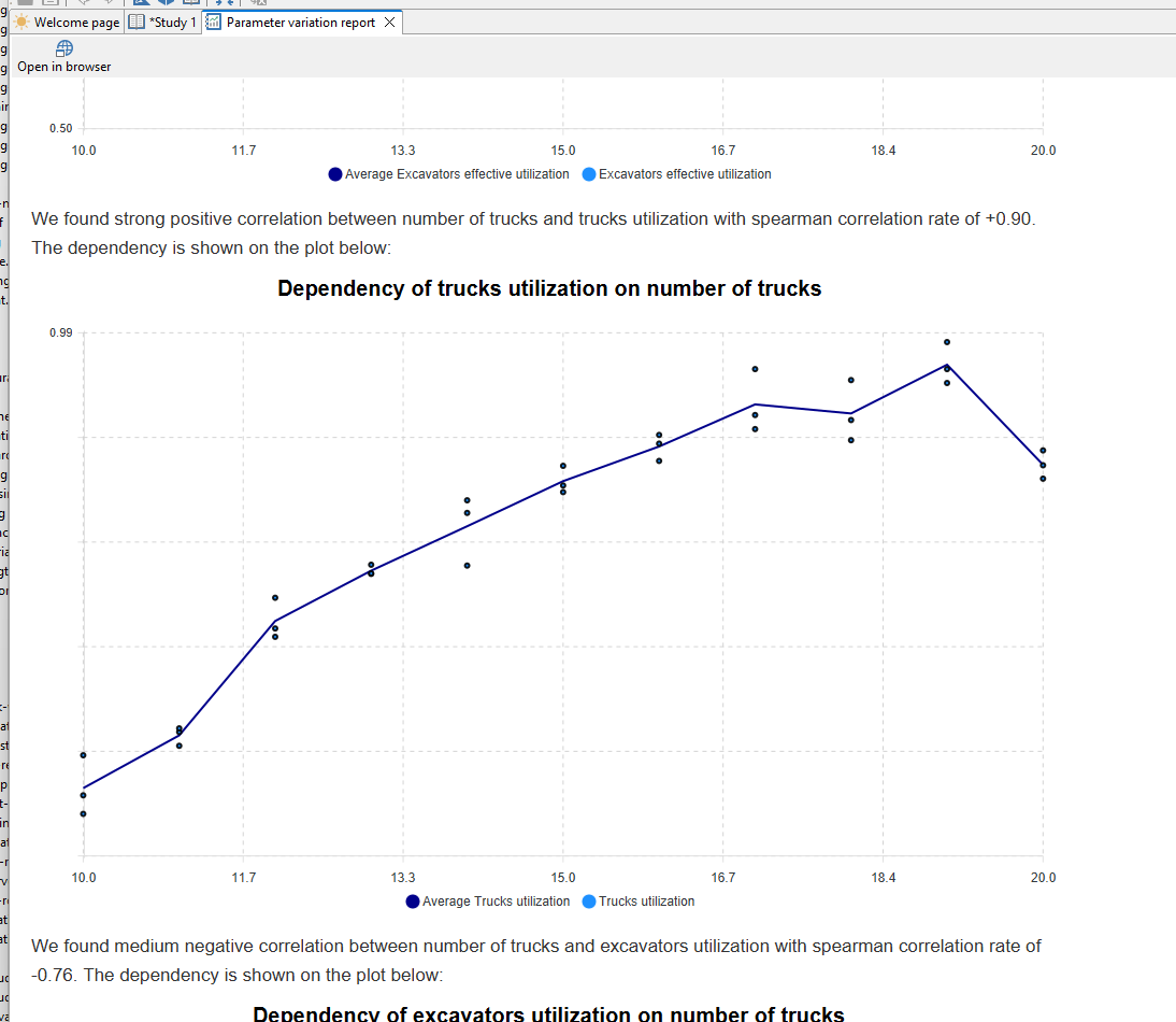
We review the updated parameter variation report. The report shows how the number of trucks correlates with key indicators under the stochastic setup, including a strong positive correlation with truck utilization and a medium negative correlation with excavator utilization. This helps us understand that adding trucks improves haulage performance, but it can also shift the bottleneck toward loading capacity.
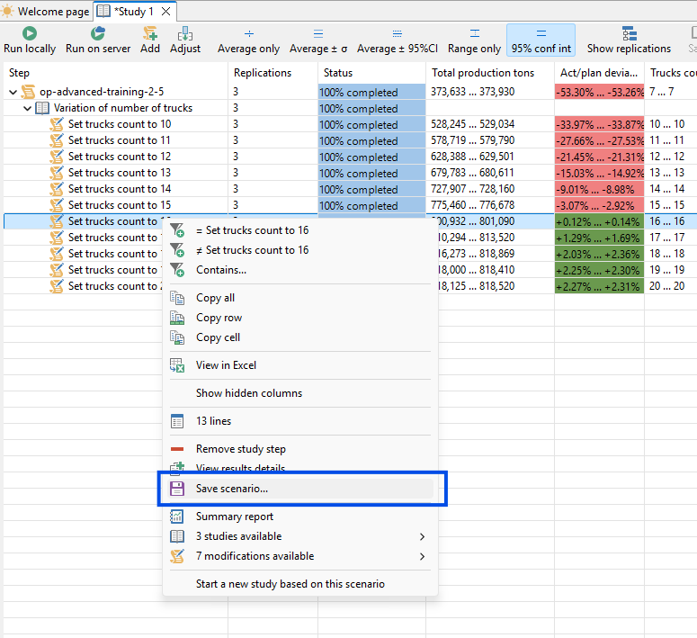
Finally, we save the selected study result as the best scenario. In the shown results, the target is reached from 16 trucks onward, so we save the scenario with 16 trucks as a balanced configuration that meets the plan without adding unnecessary extra trucks.