Import DXF and add ore and overburden blocks
1. Remove sample geometry, import DXF file and fix the data
In this section, we will replace the simple training geometry with a realistic mine layout imported from a DXF file. We will start from a prepared scenario, remove the sample map objects, and then import the pit geometry as mine arcs.
After the import, we will inspect the road network as a graph. We will use the reachability tool and graph normalization to identify disconnected fragments, split arcs at intersections, and make the imported geometry suitable for further scenario configuration.
We will be using this scenario as a base: Download scenario
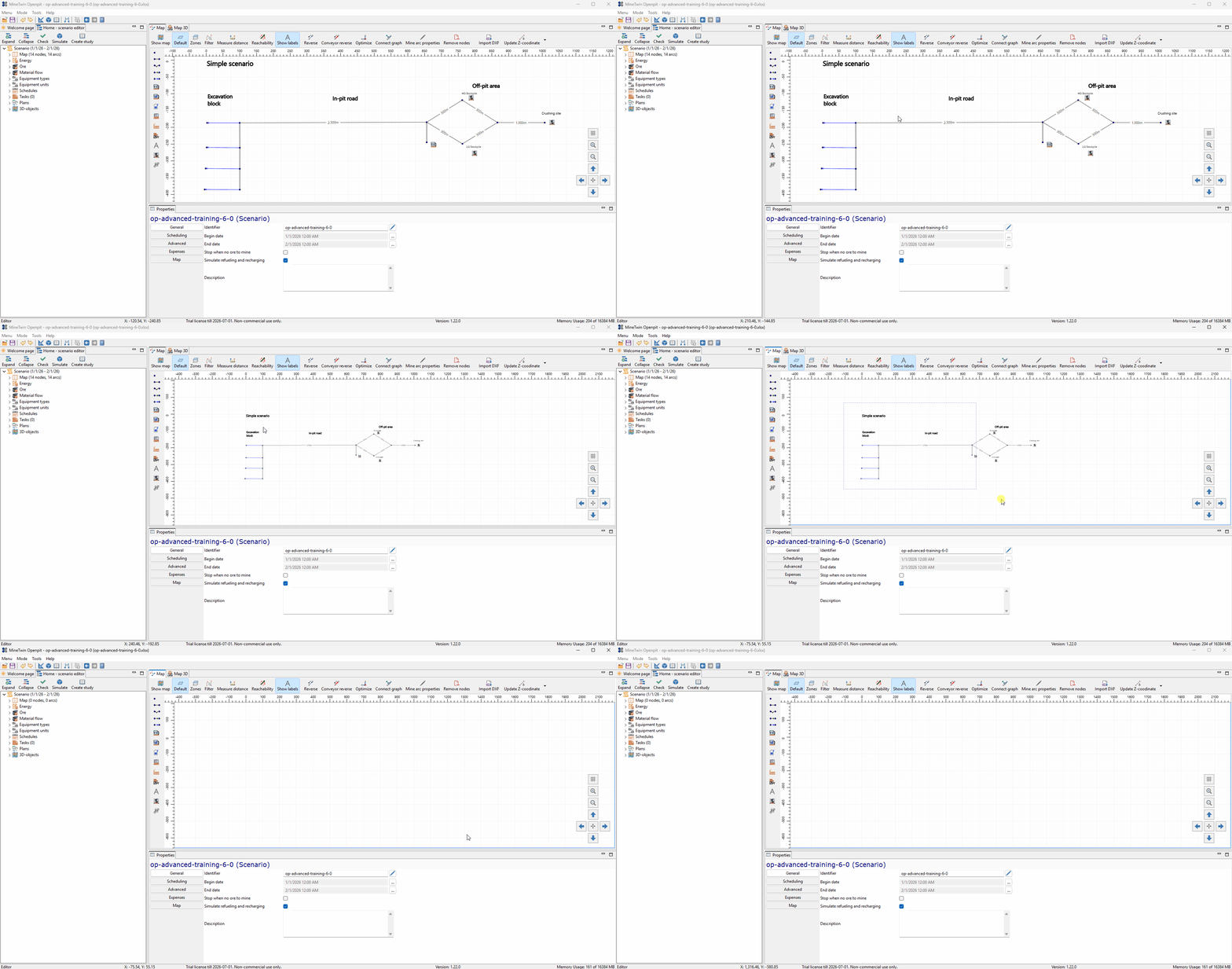
We remove the existing sample geometry from the scenario so that the map is ready for the imported DXF layout. At this point, the scenario keeps its general settings and supporting objects, while the map itself becomes empty.
We will use this sample DXF file to import the realistic geometry: Download DXF file
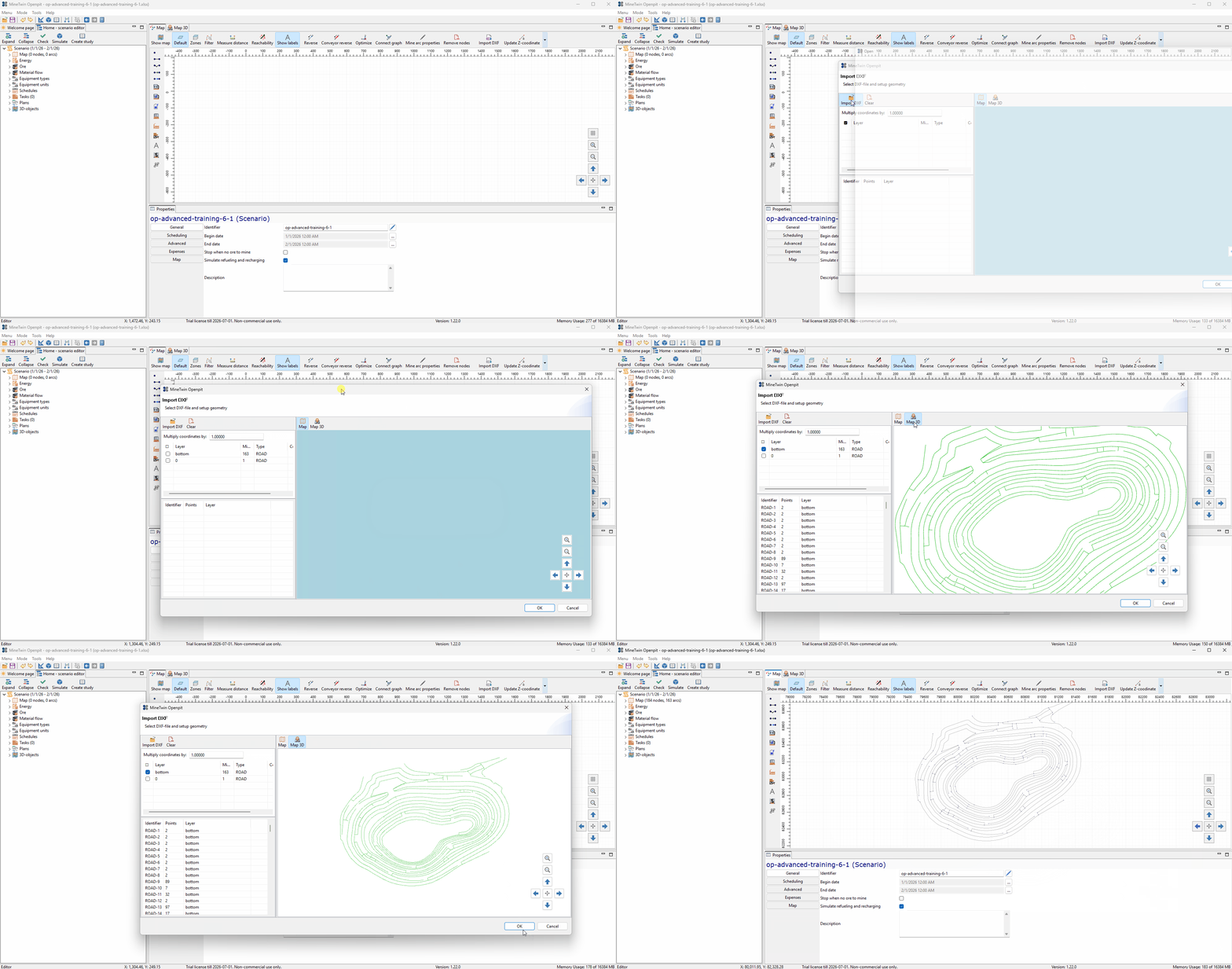
We import the sample DXF file from the map toolbar. After the import, the pit layout appears on the map as a set of mine arcs that represent the road and bench geometry from the source drawing.
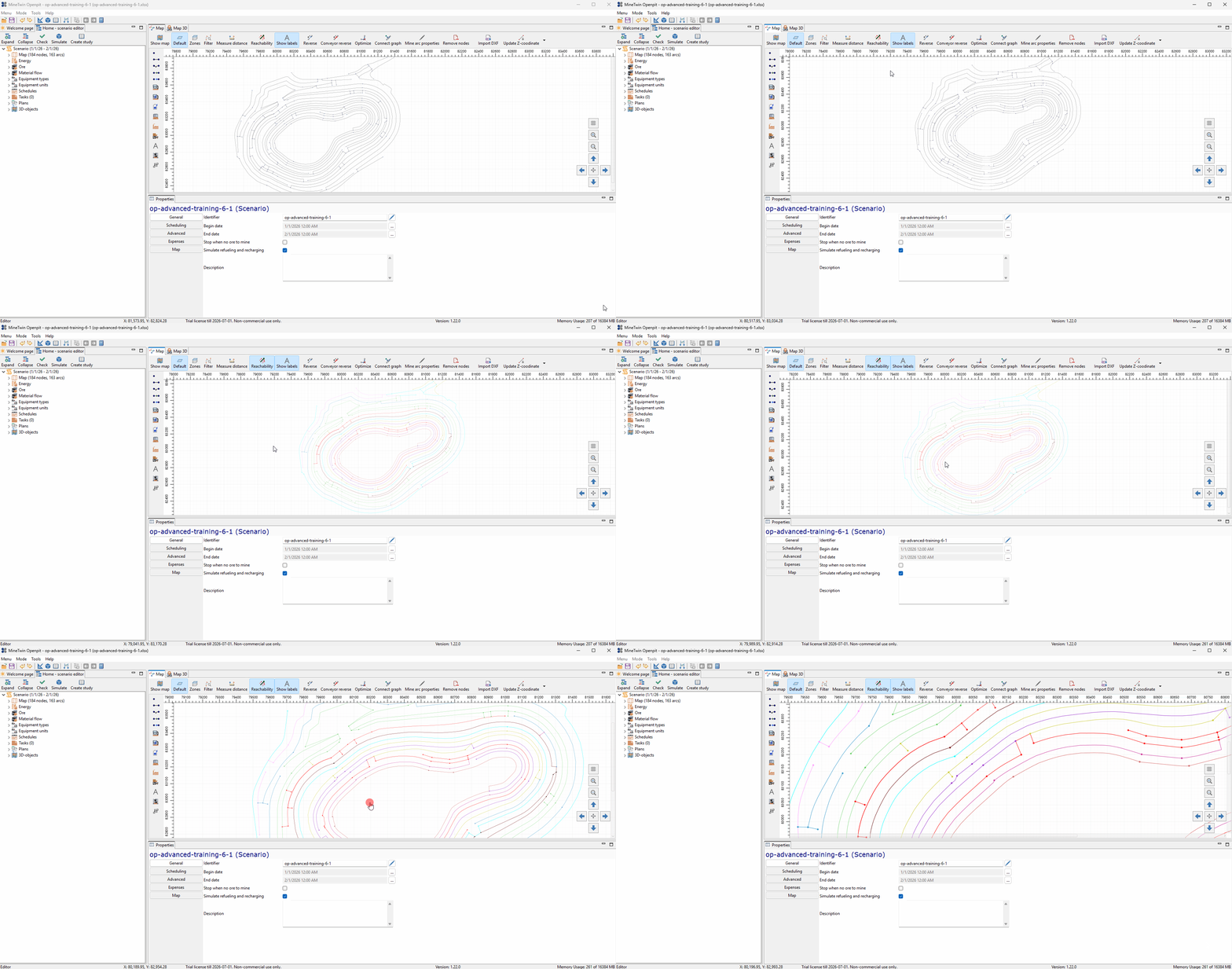
We use the reachability tool to color connected fragments of the imported network. Different colors show that the imported arcs are not yet one fully connected graph, so trucks would not be able to move freely across the whole layout.
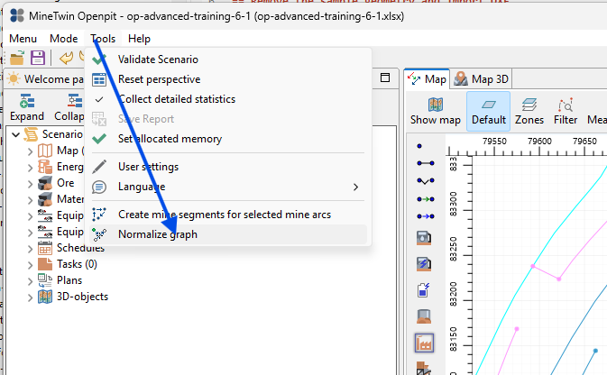
We run the Normalize graph function from the Tools menu. This function prepares the imported road graph by processing nearby nodes, near-zero-length arcs, and intersections between arcs.
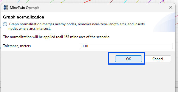
We keep the default tolerance of 0.10 meters and apply normalization to all imported mine arcs. The tolerance defines how close geometry elements must be for MineTwin to treat them as connected during normalization.
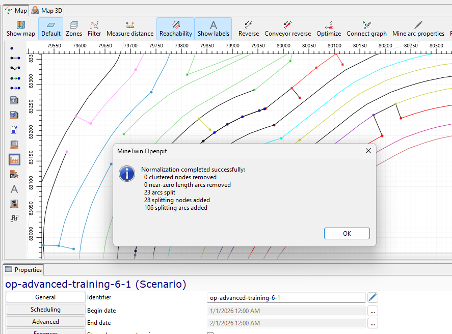
The normalization report confirms that the graph was processed successfully. In this example, MineTwin split 23 arcs, added 28 splitting nodes, and created 106 splitting arcs, which means intersections in the imported geometry were converted into usable graph connections.
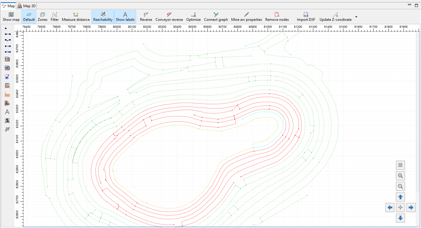
We run the reachability check again and see fewer disconnected fragments than before normalization. Some colors still remain, which means several parts of the imported network still require manual connection.
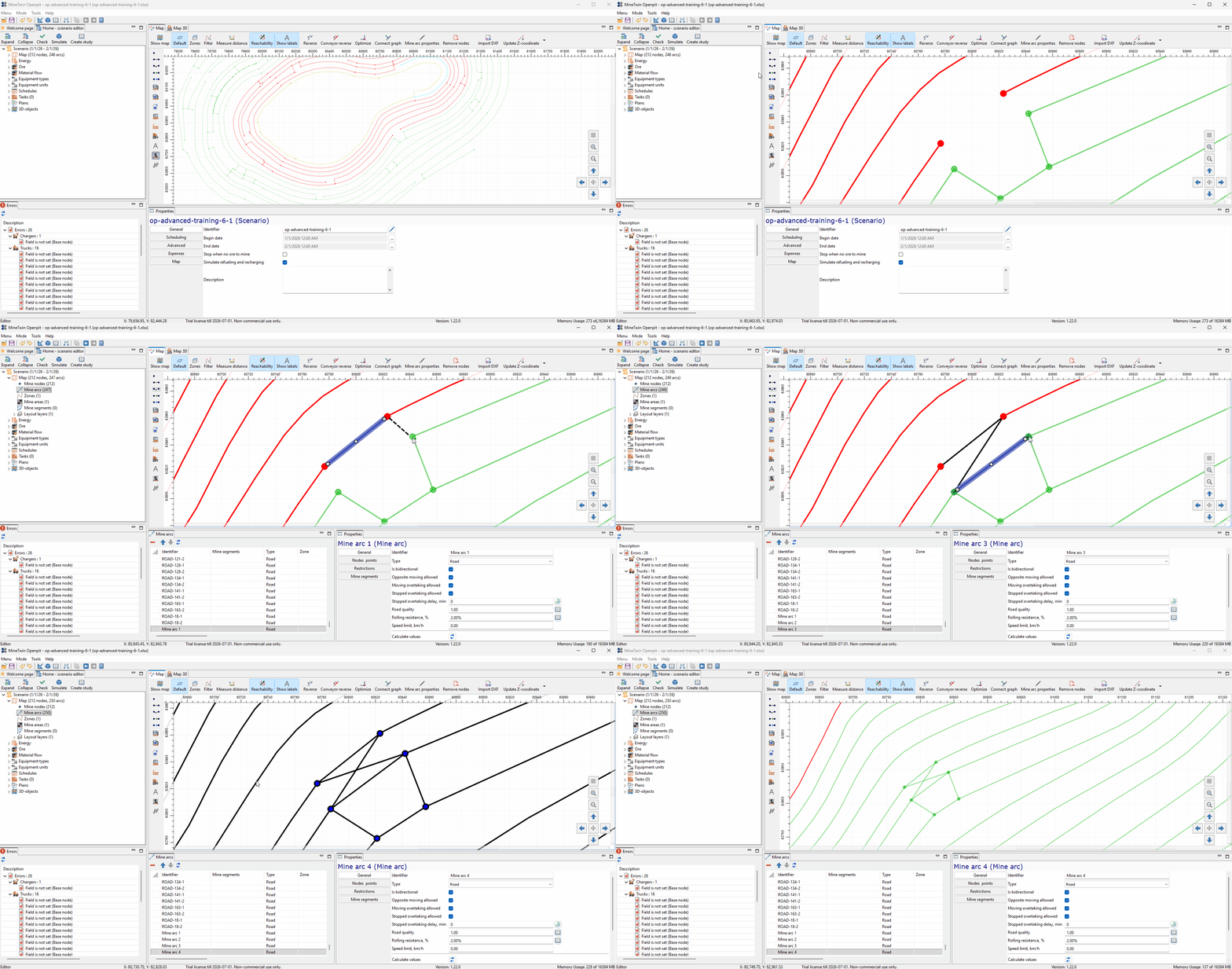
We manually connect one of the remaining disconnected fragments by adding a short connecting arc between nearby road ends. This shows the manual correction approach that we will repeat for the other disconnected parts of the imported network.
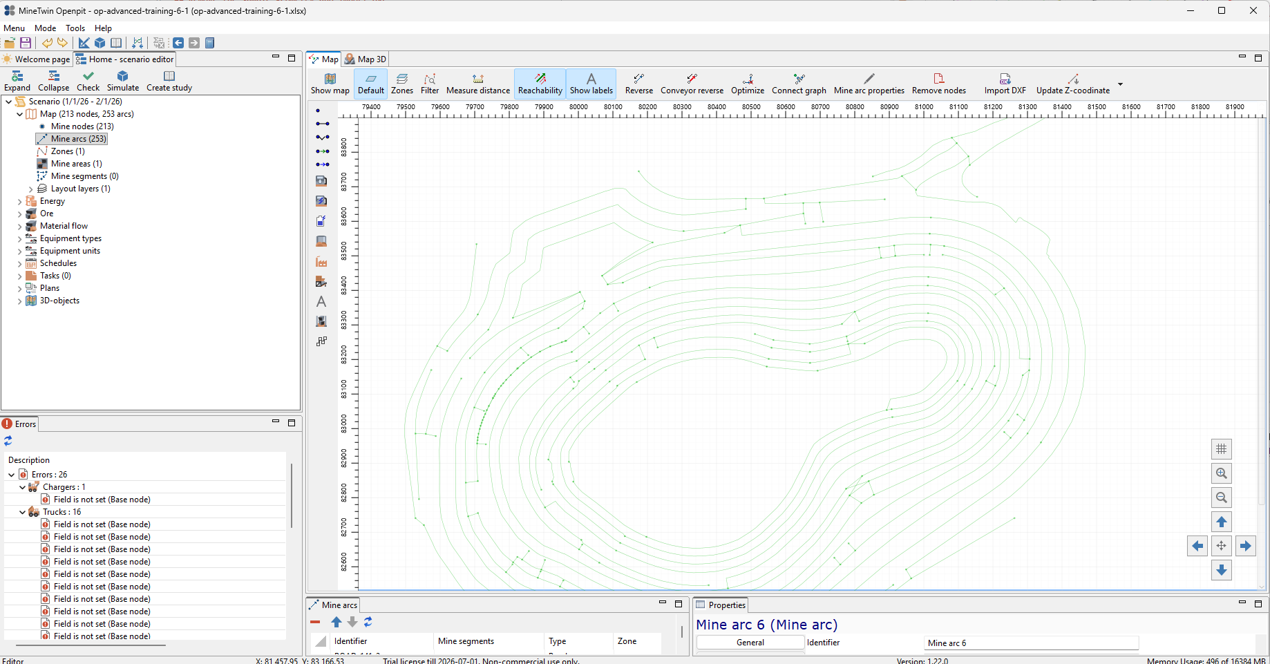
We continue connecting fragments until the reachability tool shows the network in one color. This confirms that the imported mine road graph is connected and can be used as the basis for block, destination, and equipment configuration.
2. Add ore blocks, ore destination, and base nodes for equipment
In this section, we will turn the imported geometry into a working mining scenario. We will create mine segments from selected mine arcs, configure ore blocks on these segments, and define where the mined ore should be hauled.
We will also prepare the mobile equipment for the simulation. Each equipment unit needs an initial base node, and the scenario also needs a fueling station because refueling is enabled in the scenario settings.
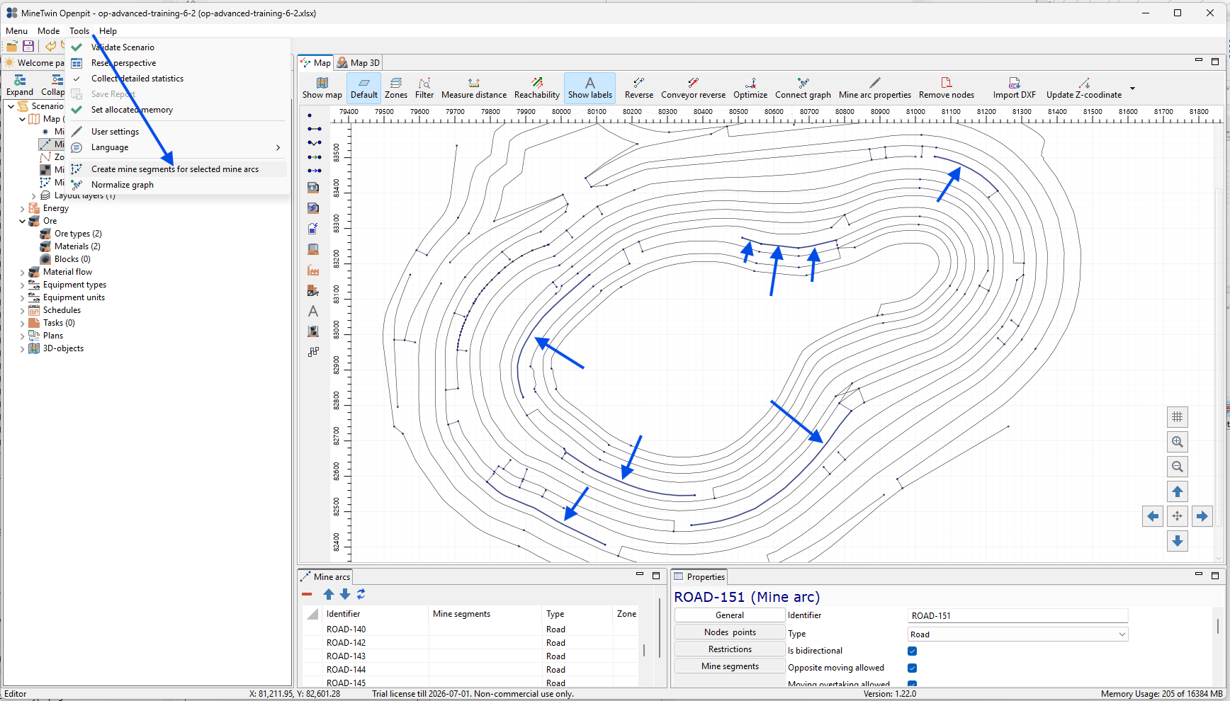
We select the mine arcs that will be used as mining fronts and run the Create mine segments function. Mine segments define the geometry along which the blocks will advance during mining.
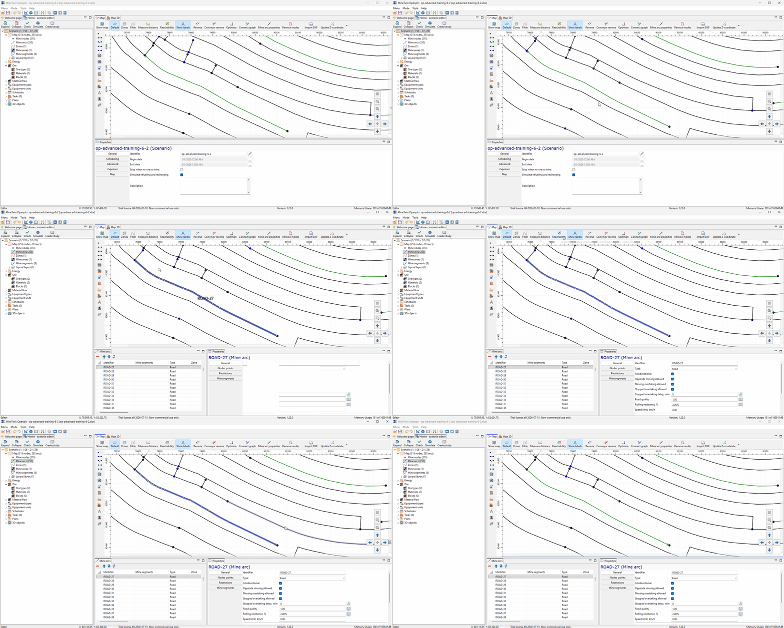
We check the direction of the created mine segments and reverse the segments where the direction is not suitable. The segment direction matters because it defines how the block advances along the selected geometry.
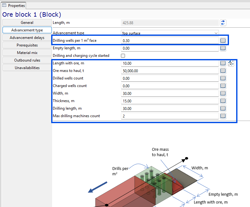
We create the first ore block and configure its advancement settings. The block uses the Top surface advancement type and receives the mining parameters shown in the blue frame, including drilling density, ore mass to haul, block dimensions, drilling length, and the maximum number of drilling machines.
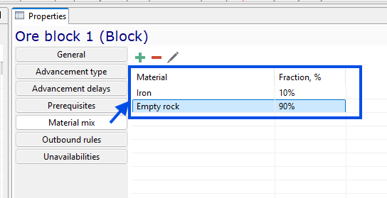
We set the material mix for the ore block. In this example, the block contains 10% iron and 90% empty rock, so its resulting quality is 10%.
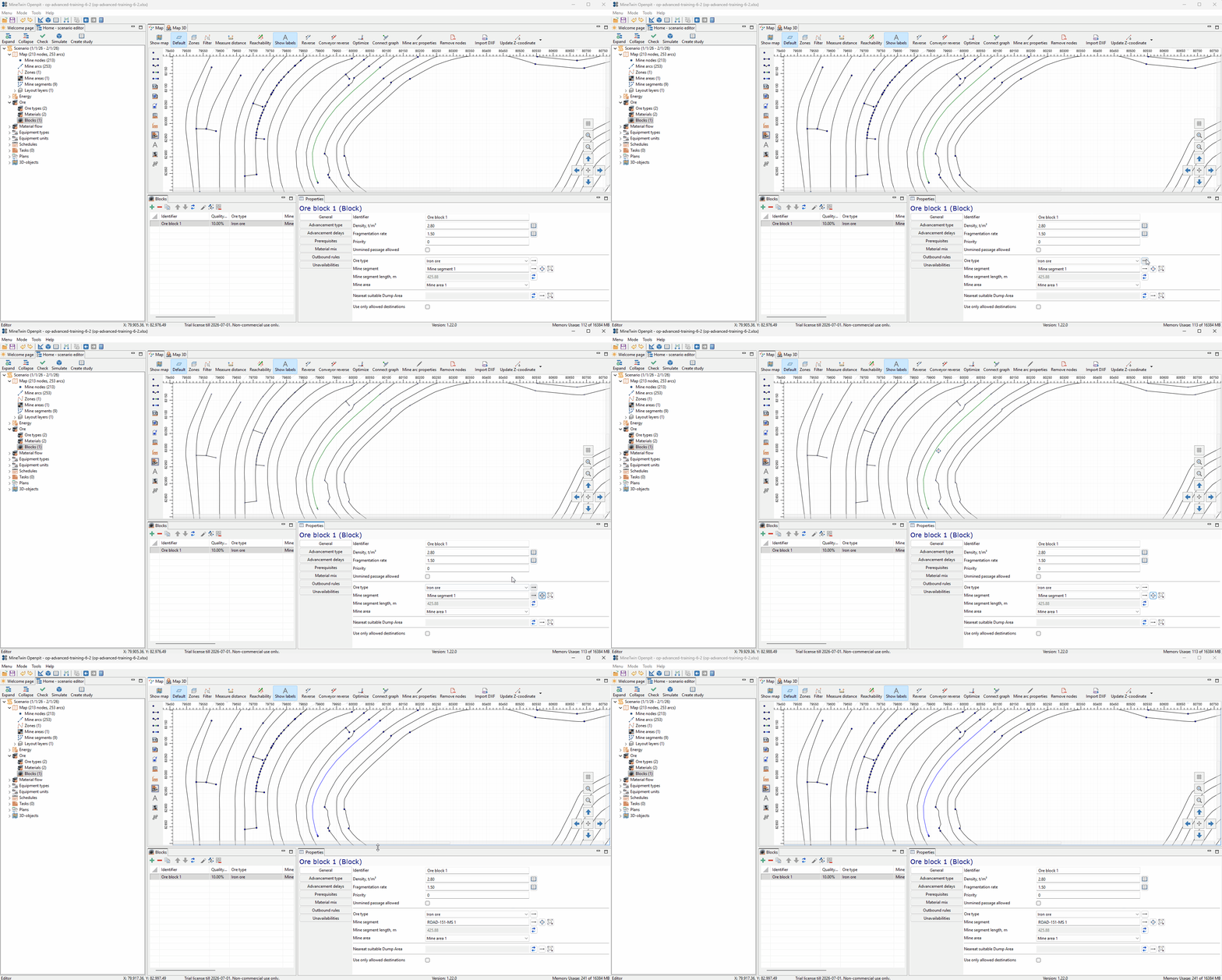
We assign a mine segment to the ore block. This connects the block configuration to the imported geometry and tells MineTwin where this block is located on the pit layout.
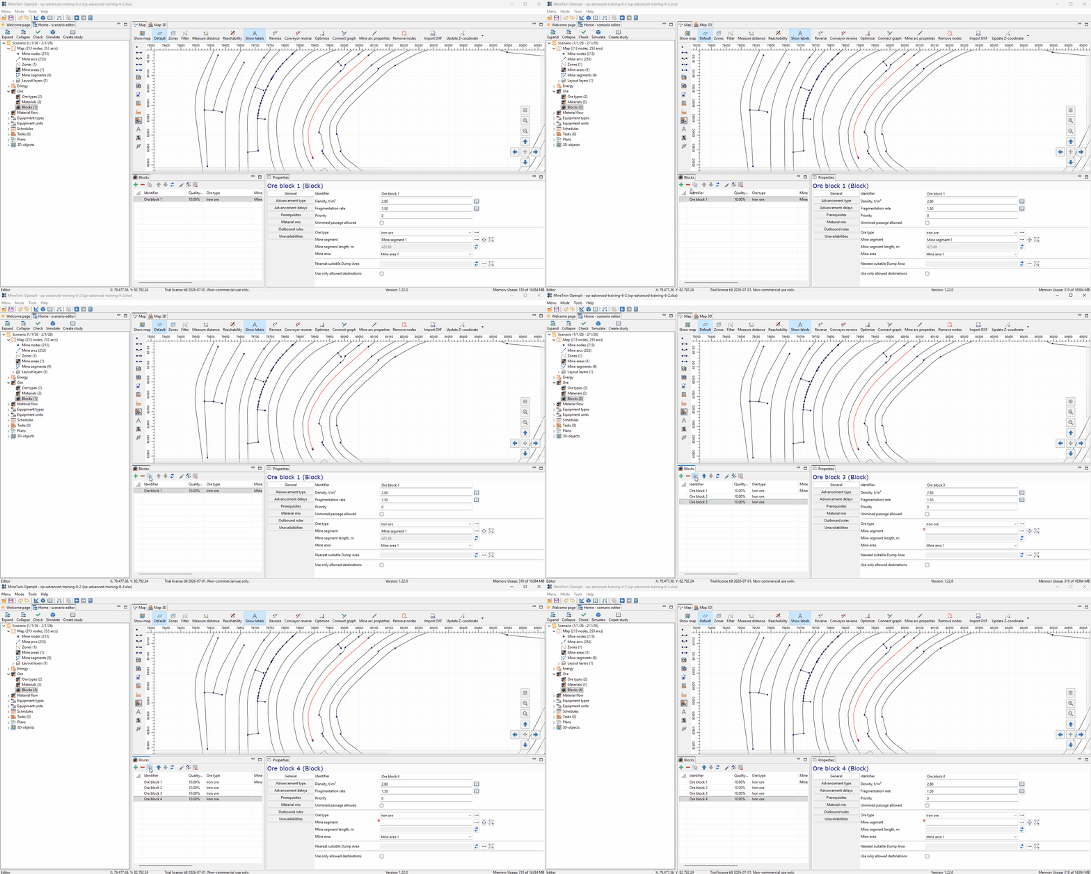
We create three additional copies of the ore block. The copied blocks keep the same main parameters and are then assigned to their own mine segments so that the scenario has four ore mining fronts.
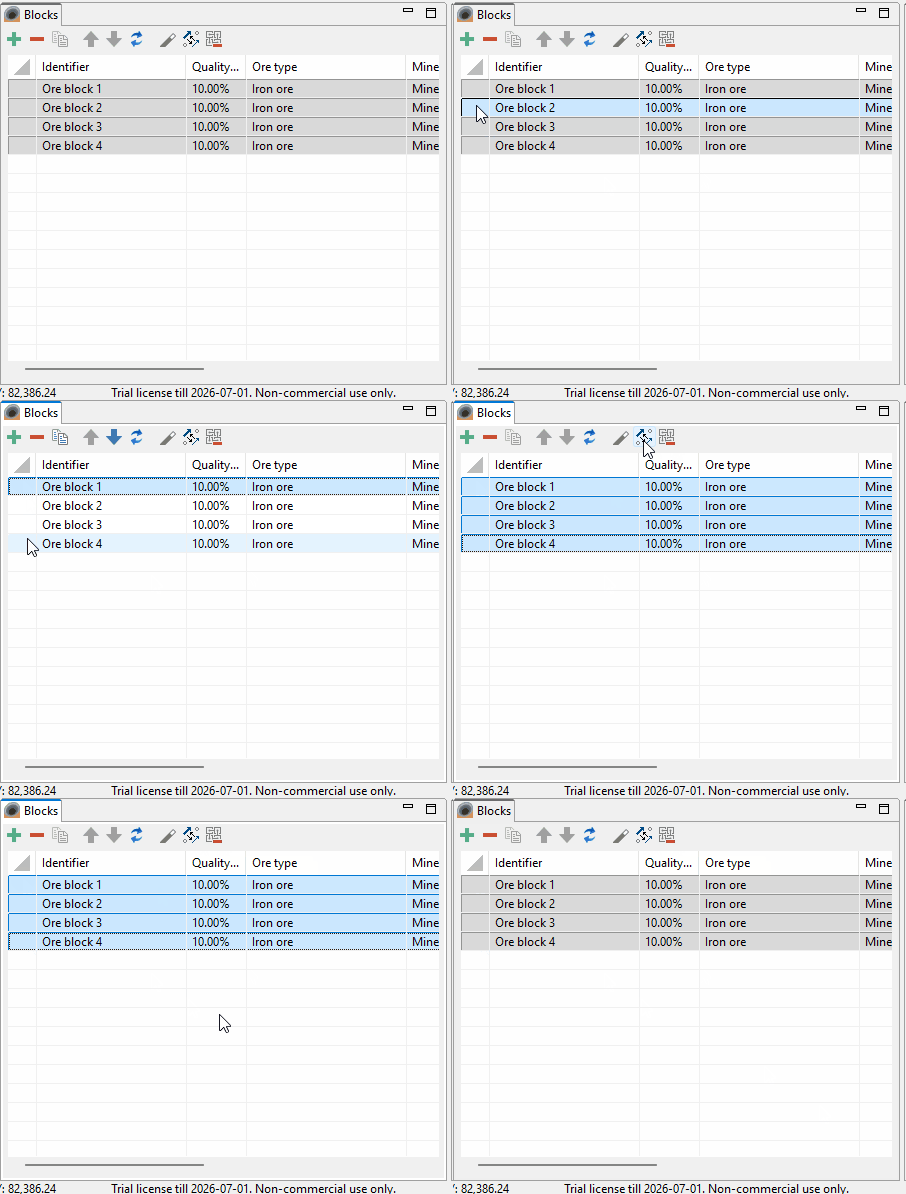
We select all ore blocks and apply the maximum length setting to them as a group. This keeps the block advancement limits consistent across all four mining fronts.
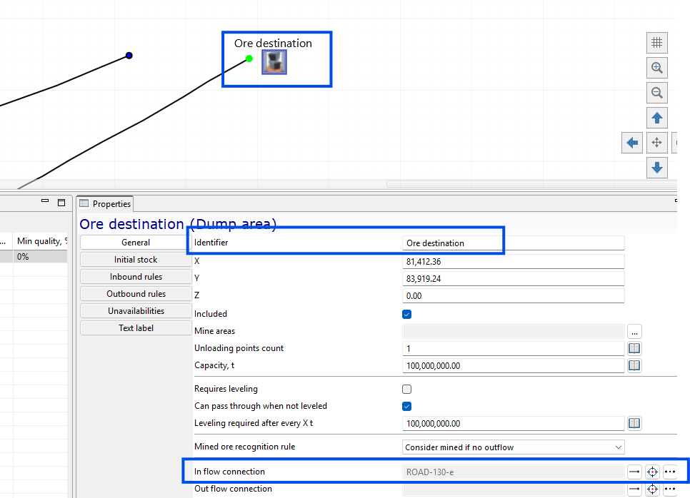
We add a dump area and name it Ore destination. This object is used as the destination for hauled ore, and its inbound connection is assigned to the road node shown in the properties.
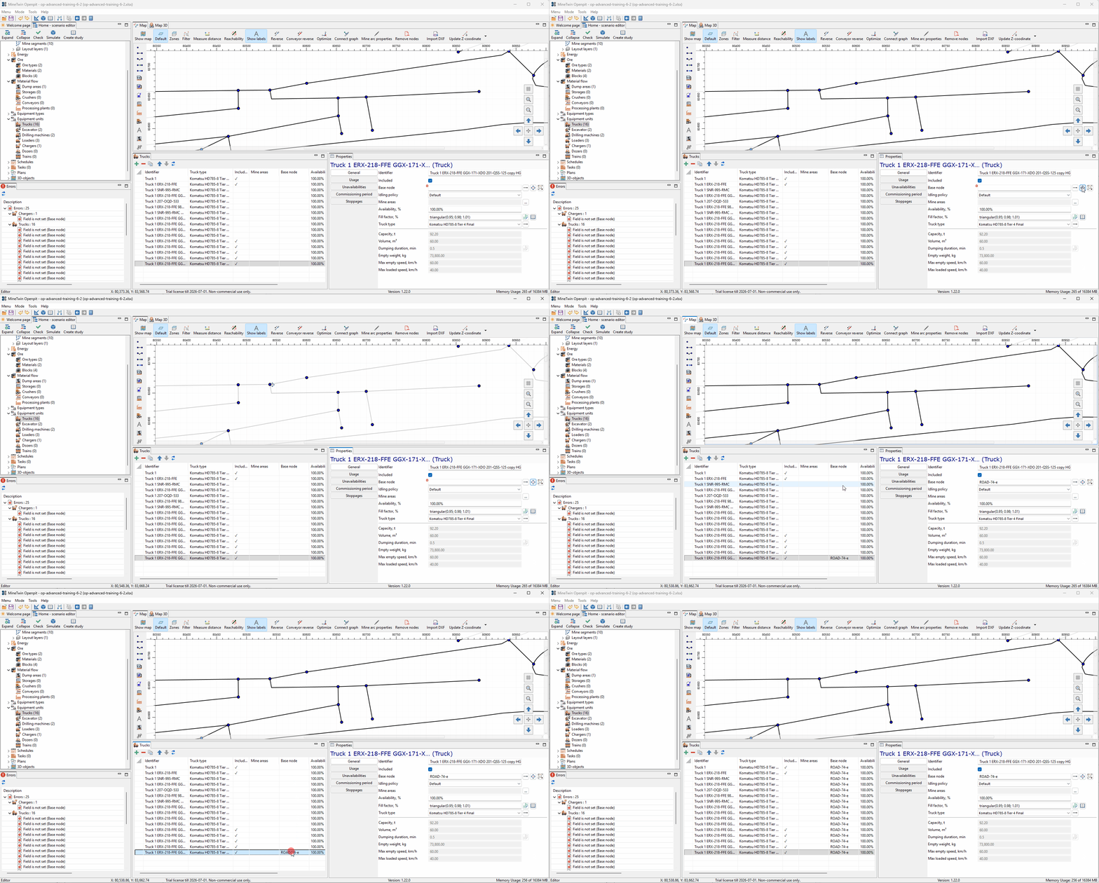
We assign base nodes to all equipment units. The base node defines the initial position of each unit at the start of the simulation.
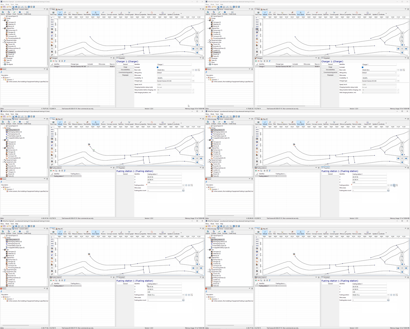
We add a fueling station and place it on the road network. Because refueling is enabled in the scenario, MineTwin needs this station to model where equipment can go for fuel.
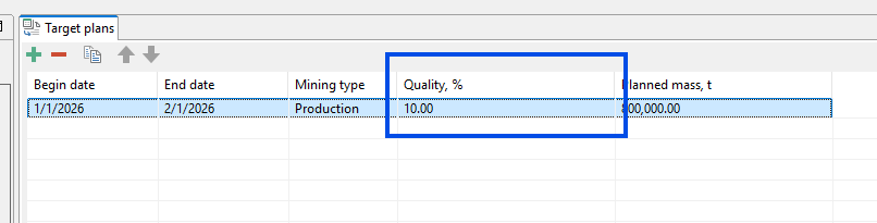
We change the production target quality to 10%. This aligns the plan with the ore blocks we created, because each block has a 10% iron quality based on its material mix.
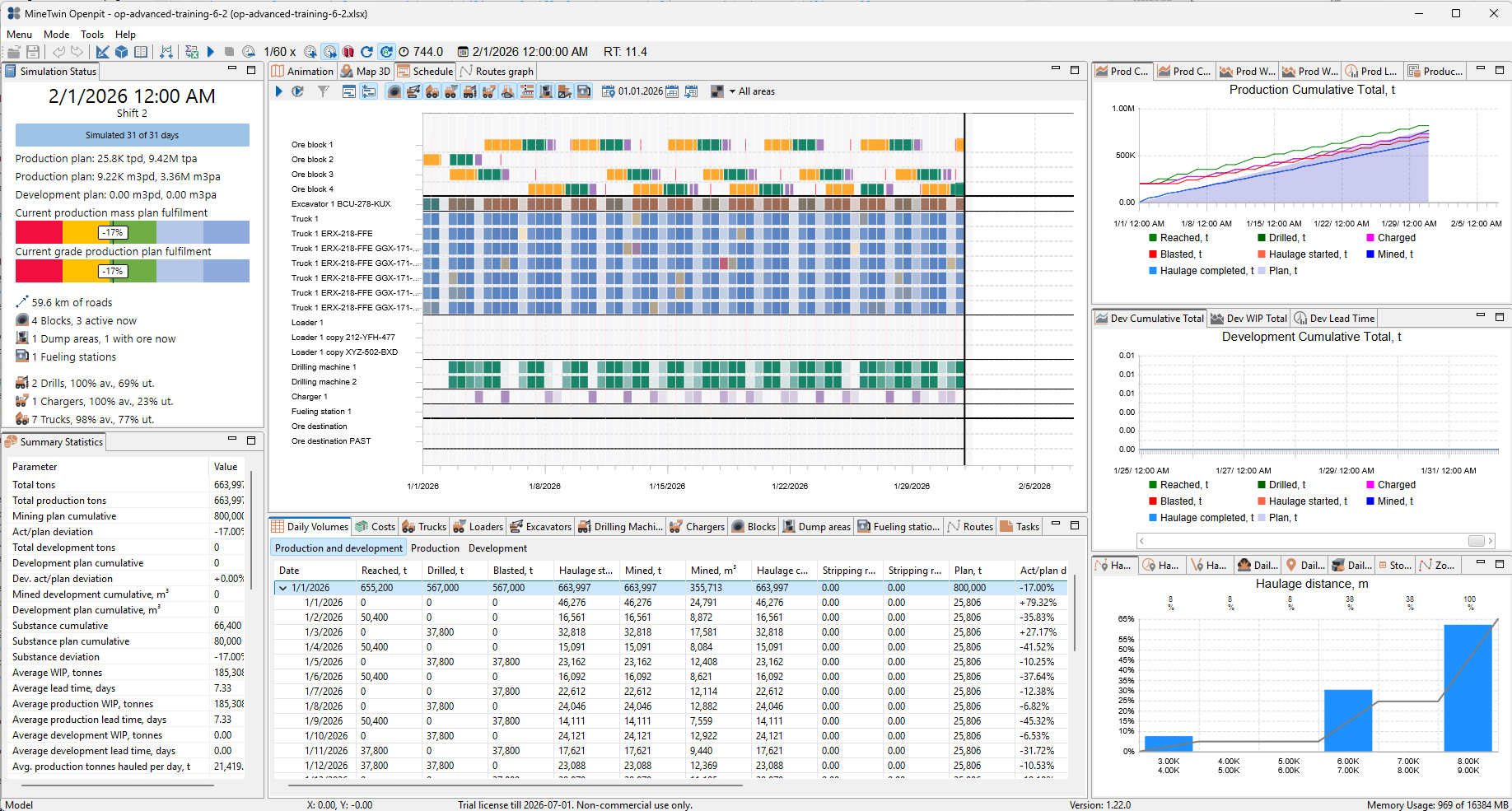
We run the simulation and review the first mining result. The schedule shows drilling, charging, blasting, hauling, and mining states for the four ore blocks, while the summary indicates that the production plan is still underfulfilled at this stage.
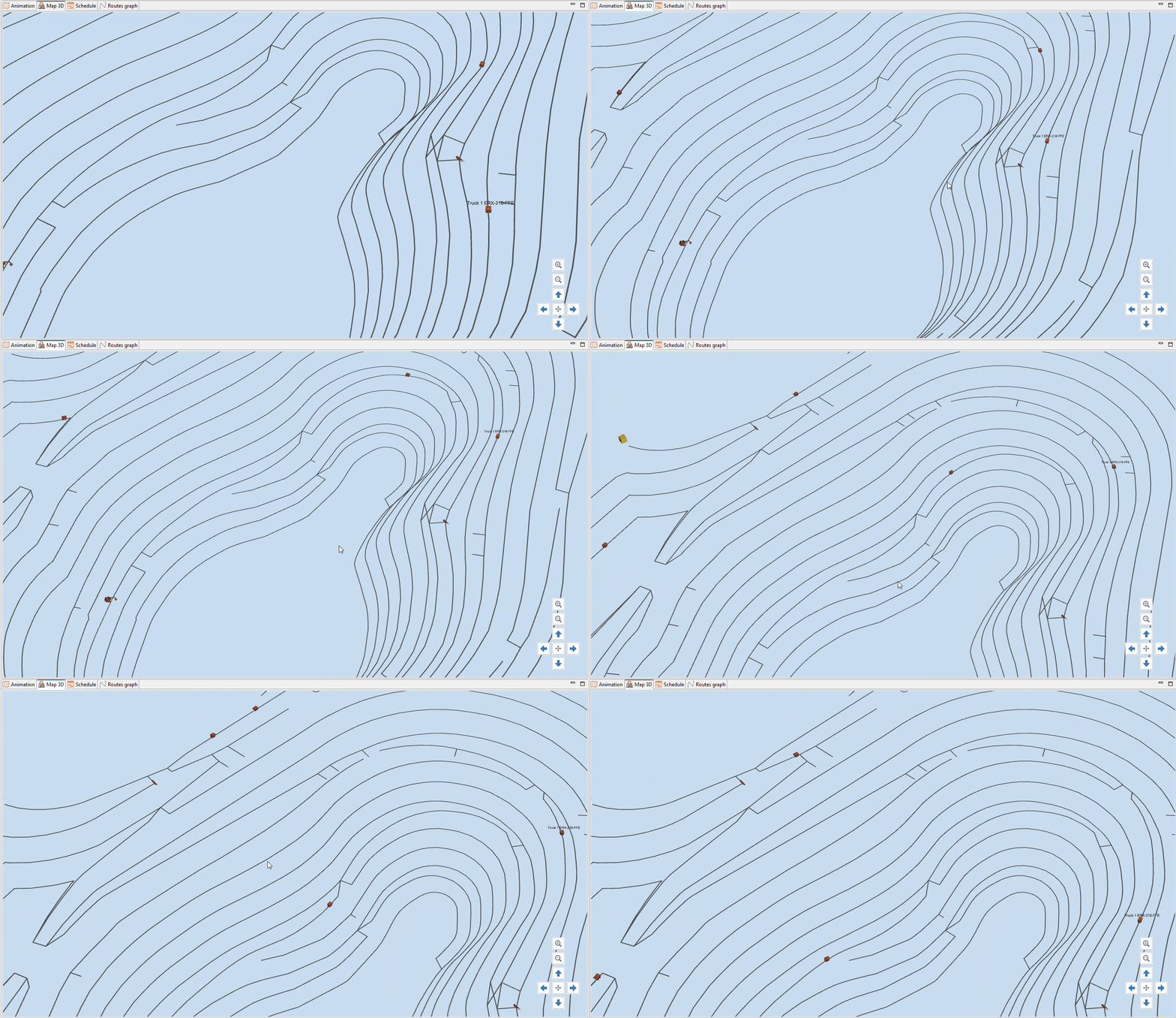
We open the 3D view and watch trucks move through the imported pit geometry. This confirms that the connected DXF-based road network is being used by the simulation and that equipment can travel through the realistic layout.
3. Add overburden blocks and overburden destination, run fleet sizing study
In this section, we will extend the scenario from ore-only mining to combined ore and overburden mining. We will add overburden blocks on separate mine segments, separate the haulage destinations for ore and overburden, and add a development target plan.
After that, we will run the simulation again and review how the production and development flows share the same road network. Finally, we will start a fleet sizing study to find a better equipment configuration for the combined plan.
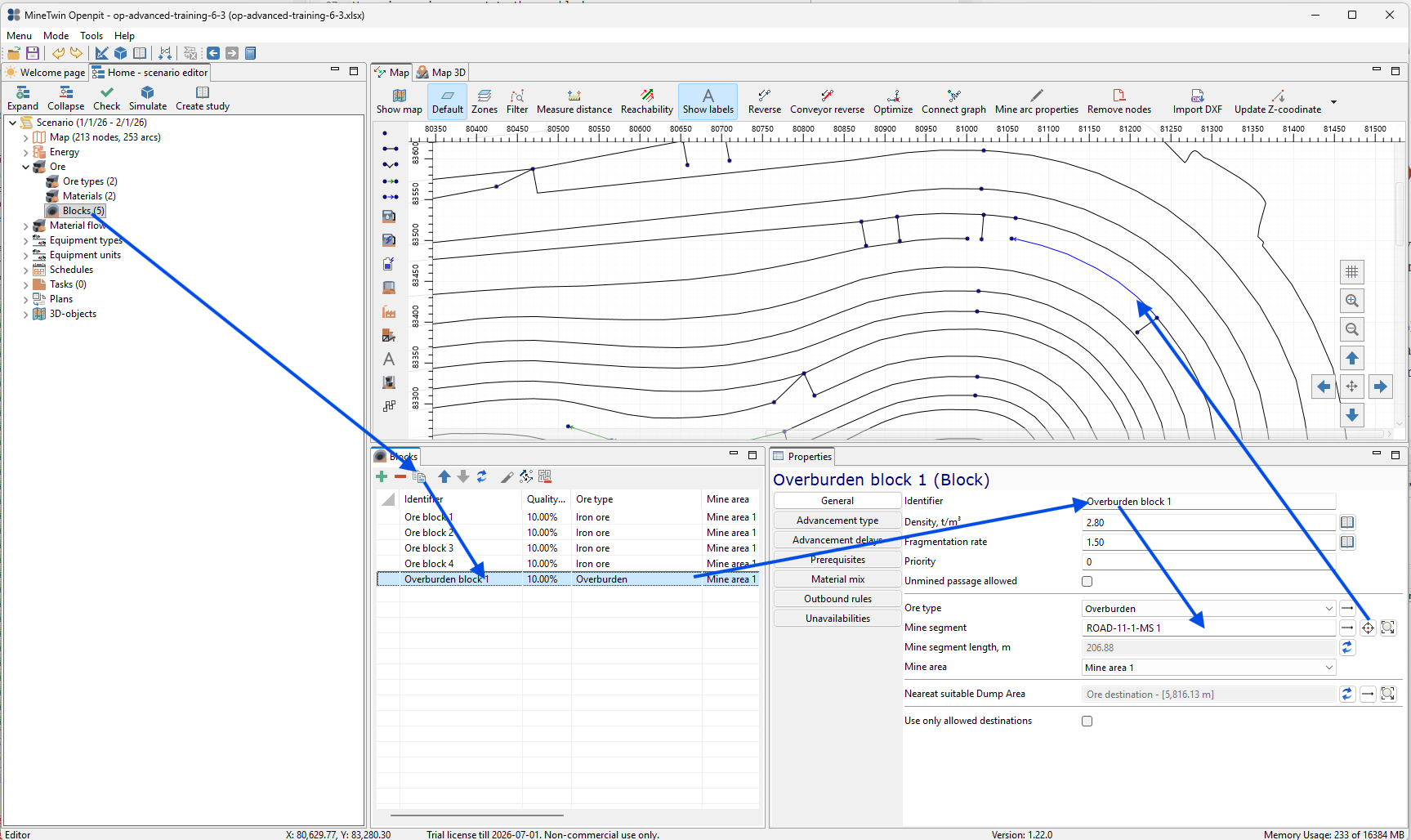
We add the first overburden block and assign it to one of the mine segments in the imported pit geometry. This creates a development mining task in the same mine area as the ore blocks.
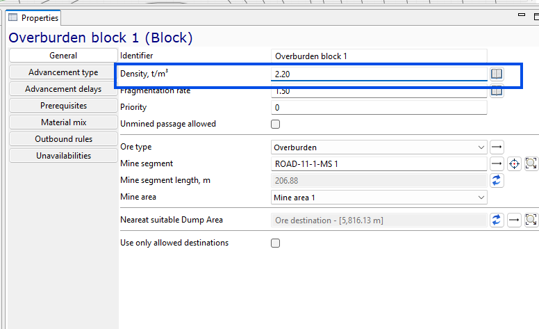
We change the overburden block density to 2.20 t/m3. This value will be used when MineTwin converts mined volume into tonnes for the development plan and haulage calculations.
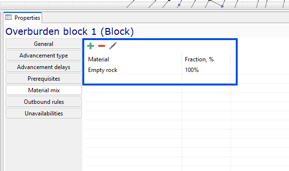
We set the material mix of the overburden block to 100% empty rock. The block is handled as overburden because its ore type is Overburden, while the material mix defines that it contains no ore material.
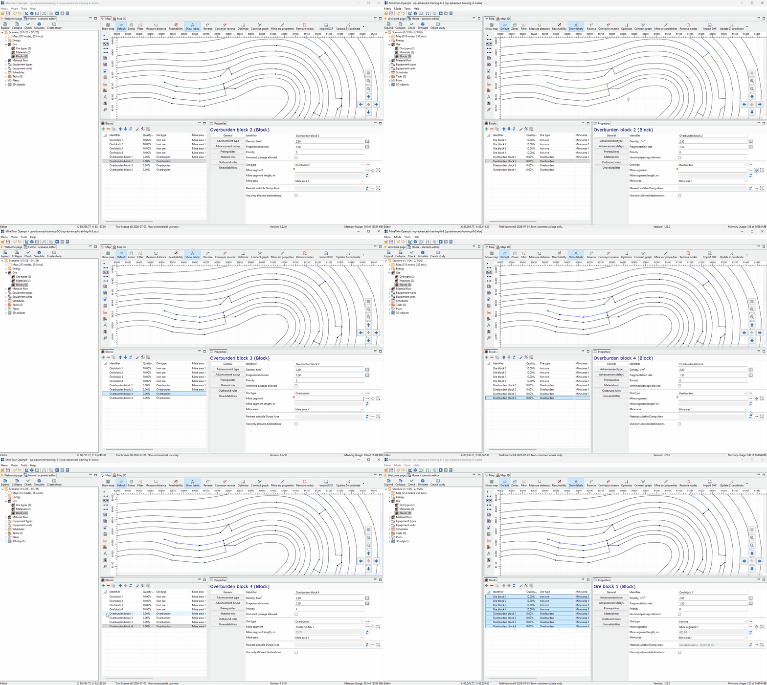
We copy the overburden block and assign the copies to their own mine segments. By the end of this step, the scenario contains four ore blocks and four overburden blocks, each linked to a specific part of the imported geometry.
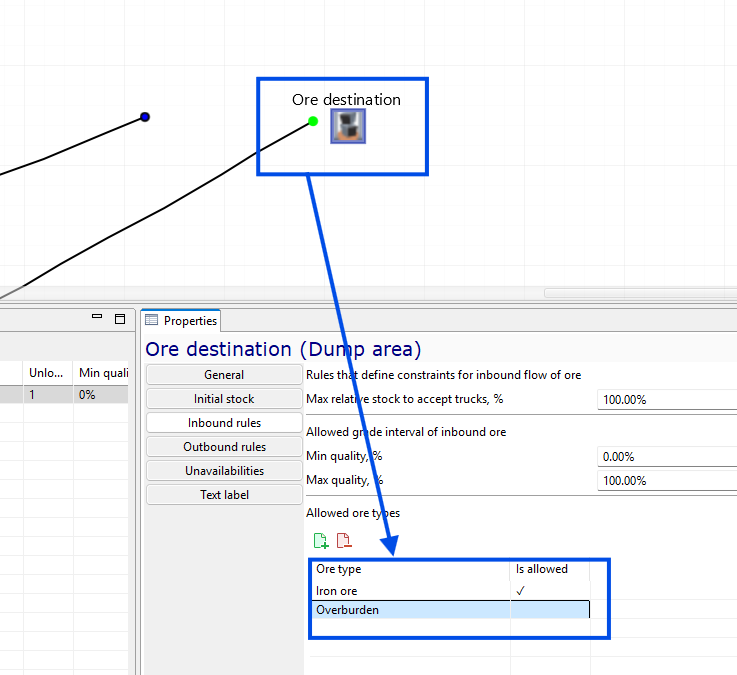
We update the inbound rules of the ore destination dump area so that it accepts only iron ore. This prevents overburden from being hauled to the ore destination.
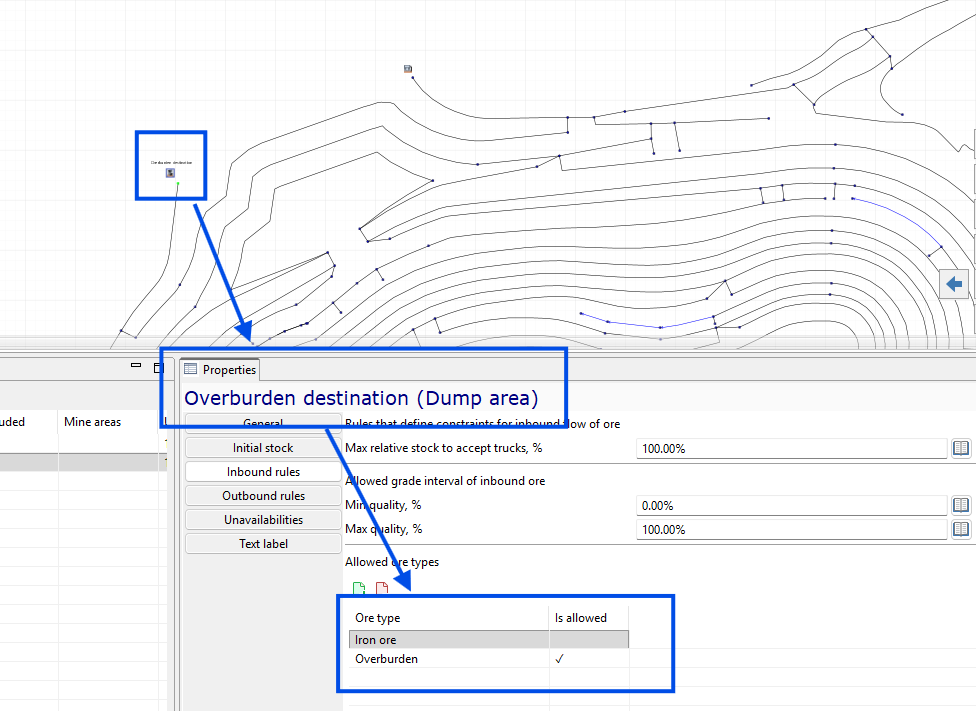
We add a separate dump area for overburden and allow it to accept overburden material. This separates production haulage from development haulage and gives MineTwin the correct destination for each material type.
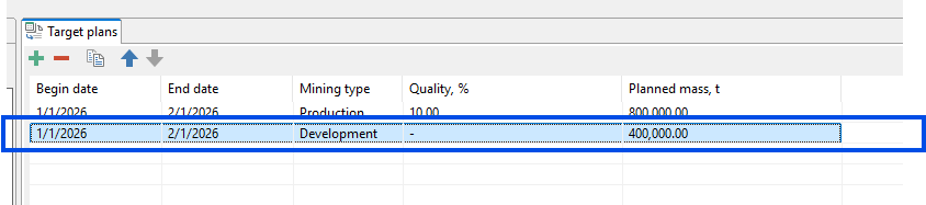
We add a development target plan for overburden. The new plan covers the same scenario period and sets the planned development mass to 400,000 tonnes.
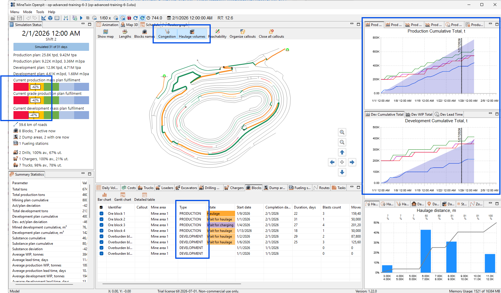
We run the simulation and review both production and development results. The dashboard now shows eight blocks, two dump areas, and separate fulfillment indicators for production mass, production grade, and development mass. We also enable the Congestion and Haulage volumes layers on the map to see where the active haulage routes are loaded.
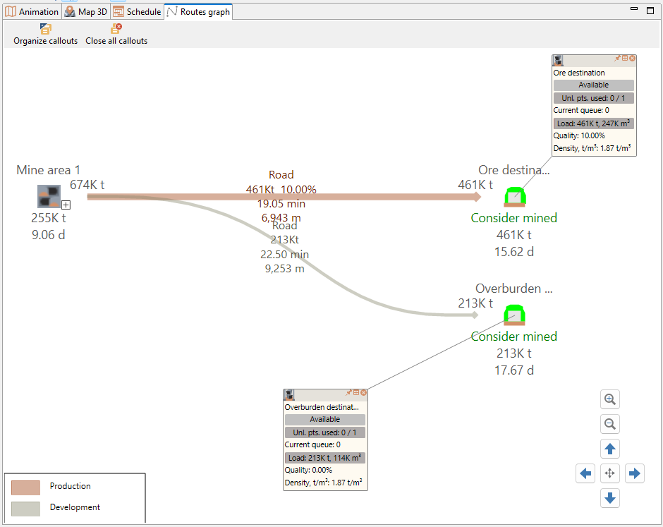
We open the routes graph to compare ore and overburden flows. The graph shows ore hauled to the ore destination and overburden hauled to the overburden destination, with different route distances and travel times through the same mine area.
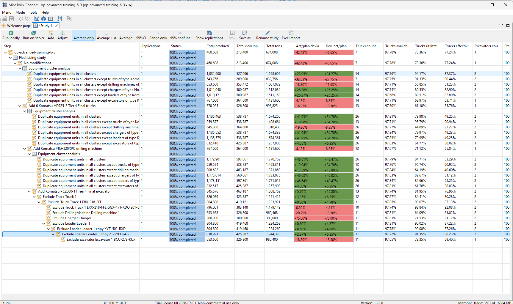
We run a fleet sizing study for the combined production and development scenario. The study evaluates equipment clusters, adds equipment where it improves plan fulfillment, and then tests exclusions to remove equipment that is not needed for the final configuration.
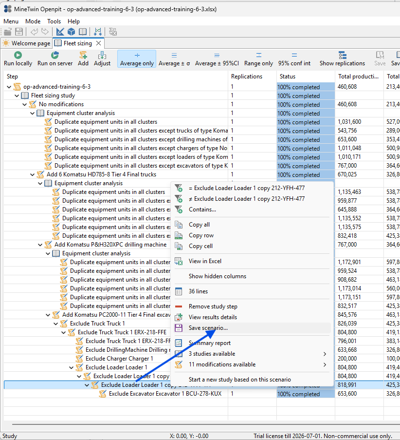
We select the best study result and save it as a new scenario. This gives us a scenario variant with the equipment configuration chosen by the fleet sizing study.