Add more realism and do scenario analysis

In this section, we will add fuel consumption and refueling behavior to the scenario. We will switch on refueling simulation, add a fueling station near the depot, correct the depot node elevation, and then run the model to review the truck fuel plots.

This makes the scenario more realistic because trucks will no longer be treated as if they can operate without fuel constraints. MineTwin will track fuel levels, send equipment to a fueling position when needed, and include refueling time in the simulated operation.

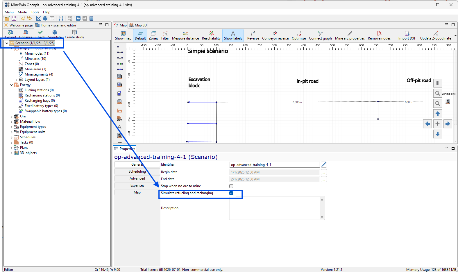
We switch on simulation of refueling and recharging in the scenario properties. According to the MineTwin scenario settings, when this option is enabled, refueling is simulated instead of only calculating fuel demand.

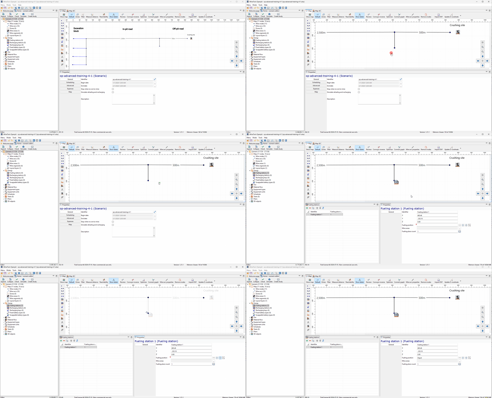
We add one fueling station near the depot and set its fueling position to the Depot node. A fueling station is stationary equipment used for refueling transport and equipment units, and the fueling position defines where a unit stands while refueling.

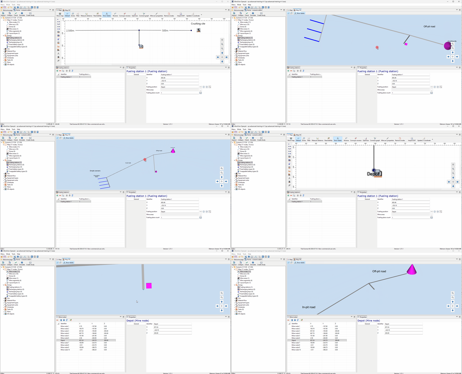
We correct the Z coordinate of the Depot node to 200 m. This is important because node elevations are used to calculate road gradients, which affect truck movement and fuel consumption.

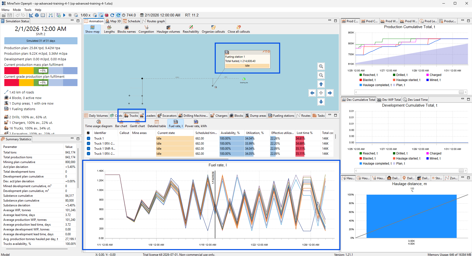
We run the simulation and review the fuel-related outputs. The animation callout shows the fueling station status and total fuel consumed, while the truck Fuel rate plot shows how fuel levels change during the month as trucks work and return for refueling.

Download scenario

In this section, we will allow several drilling machines to work on the same block at the same time. The scenario already has two drilling machines, but the block settings still need to allow parallel drilling work.

This change helps us model a more realistic and more flexible drilling process. Instead of forcing one drilling machine to complete the whole drilling scope alone, MineTwin can split the drilling work between available machines when the block configuration allows it.

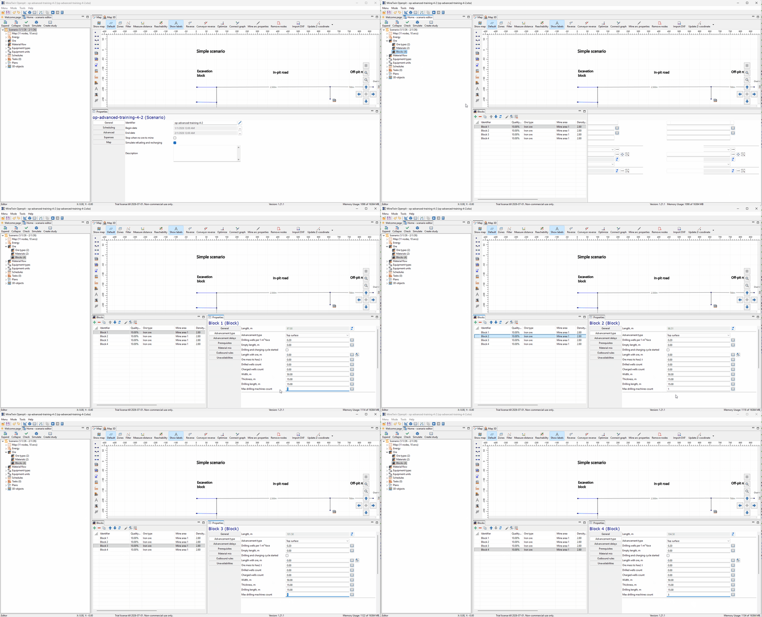
We set the Max drilling machines count parameter to 3 for the blocks. This parameter defines how many drilling machines are allowed to work on one block in parallel, so the two available drilling machines can now be assigned to the same block when needed.

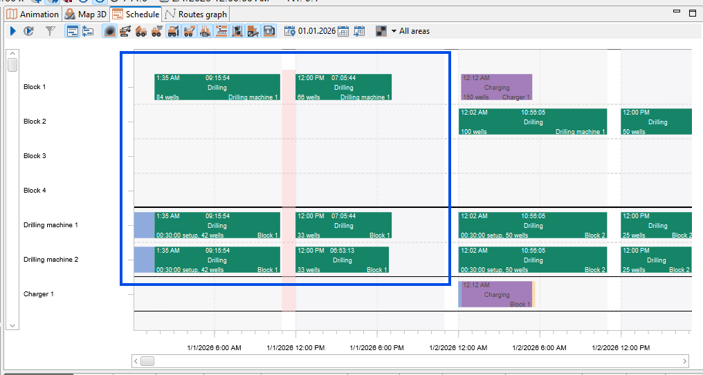
We run the simulation and review the Gantt chart. The chart shows Drilling machine 1 and Drilling machine 2 working on Block 1 at the same time, with the drilling scope split between them before the block moves to charging.

Download scenario

In this section, we will add planned maintenance and unplanned truck failures. We will create an inspection maintenance set, assign it to the truck type, then add a flat tyre event as a random unplanned downtime.

This lets us model that trucks are not only limited by shifts, queues, and fuel. They can also become unavailable because of scheduled inspections or random failures, and these periods will affect availability, utilization, and effective utilization.

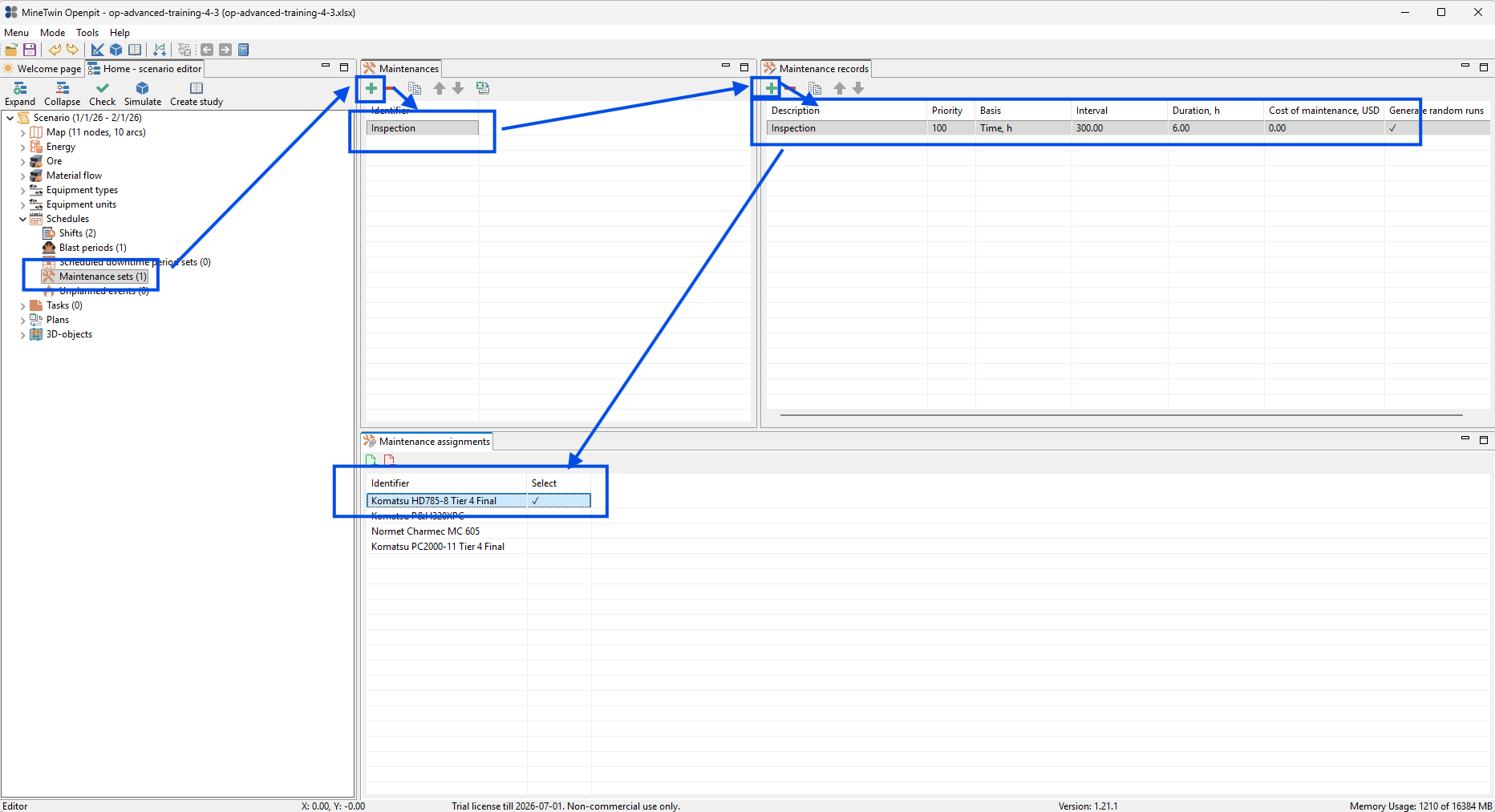
We create a maintenance set named Inspection and add a maintenance record for the truck type. The inspection is triggered every 300 operating hours, lasts 6 hours, and is assigned to the Komatsu HD785-8 truck type. The Generate random runs option is enabled, so inspections are distributed across truck units instead of occurring for all trucks at the same time.

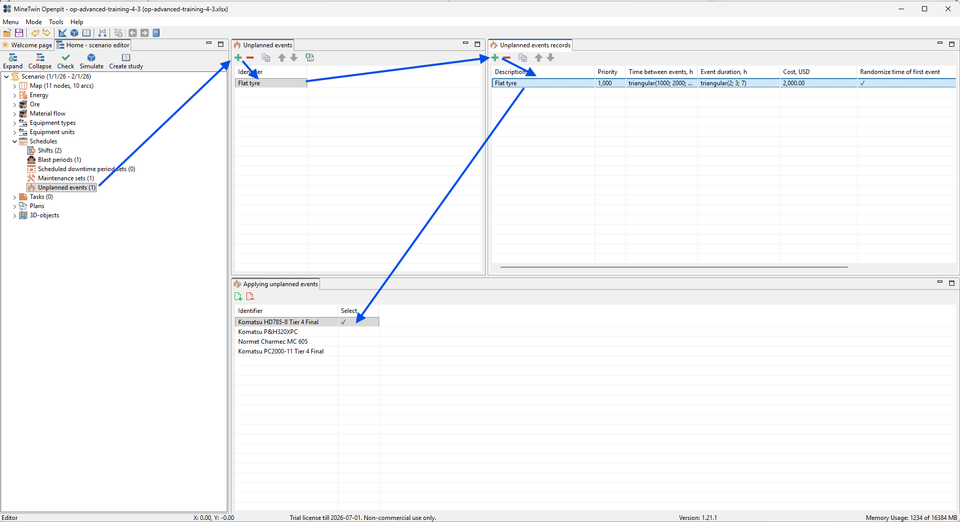
We add an unplanned event named Flat tyre and assign it to the same truck type. This event represents random truck downtime caused by a tyre failure, with the event timing and duration defined in the unplanned events record.

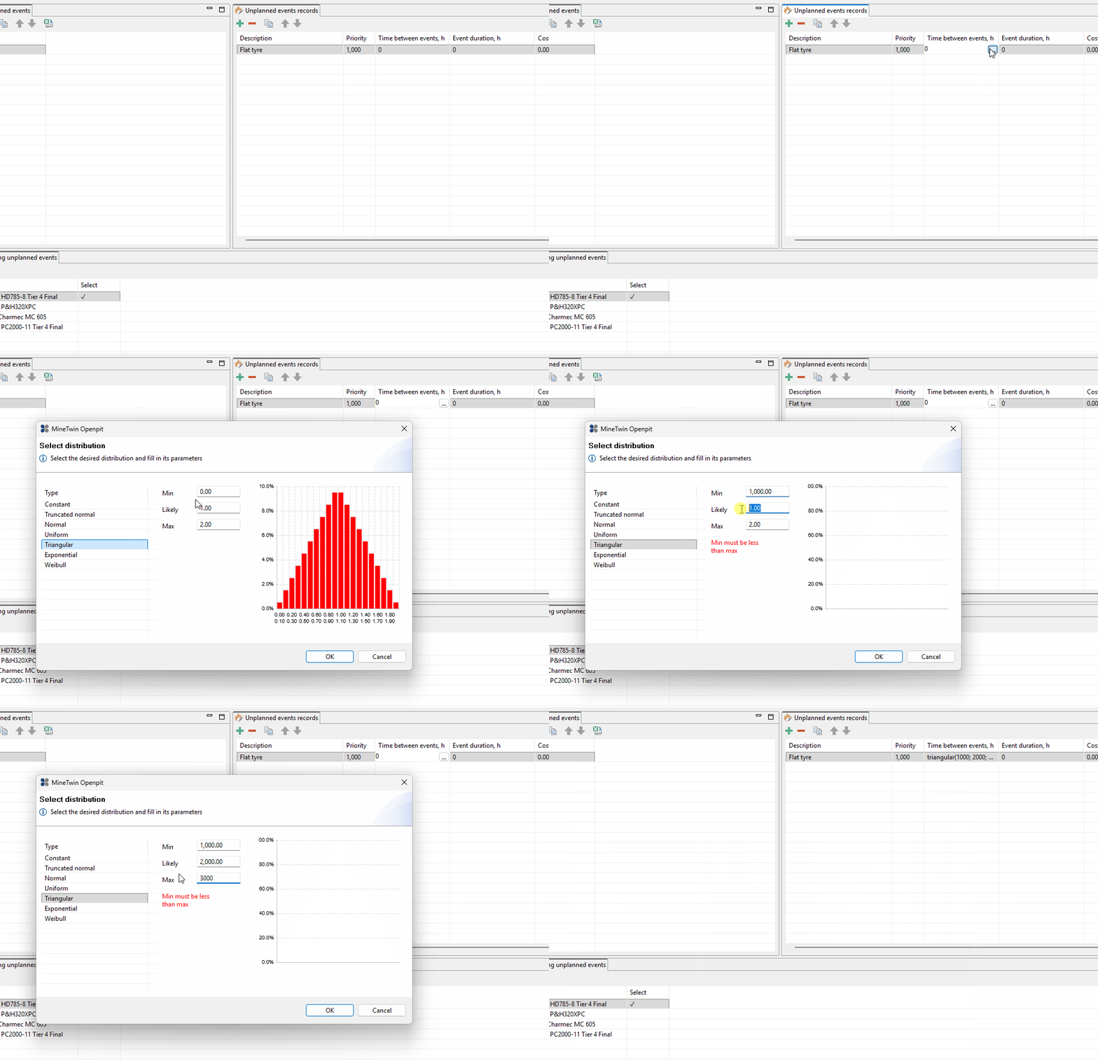
We change the time between flat tyre events from a fixed value to a triangular distribution. This makes the failure process stochastic, so different replications can produce different failure moments instead of repeating the same downtime pattern.

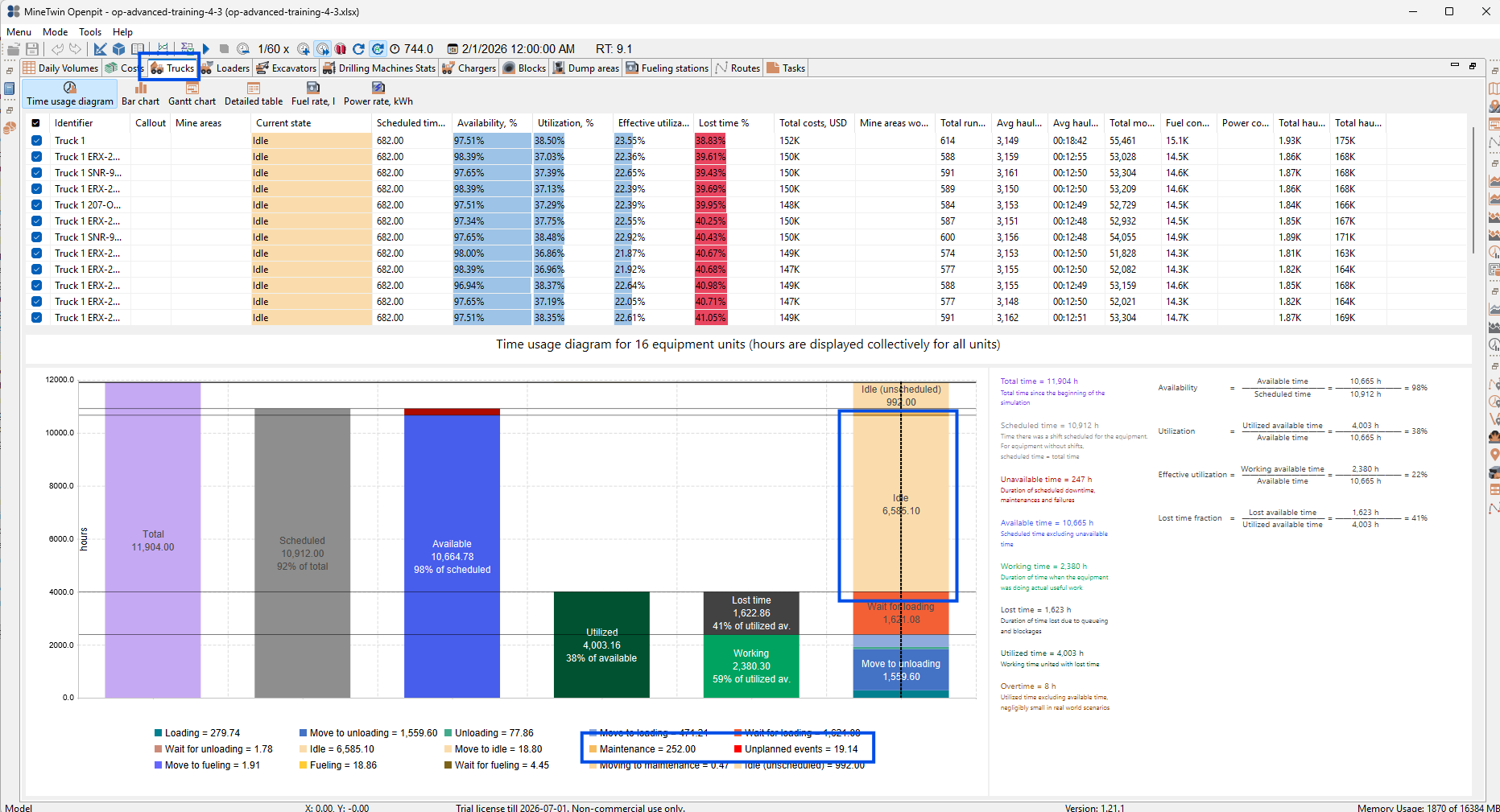
We run the simulation and review the truck time usage diagram. The diagram now includes Maintenance and Unplanned events categories, which reduce truck availability by adding unavailable time. The truck table also helps us compare utilization and effective utilization after maintenance and failures are included.

Download scenario

In this section, we will rerun Fleet sizing after adding fuel, maintenance, failures, and parallel drilling. We will use five replications so the study evaluates fleet configurations under variability instead of relying on one deterministic simulation run.

The goal is now different from the first fleet sizing study. The current scenario already reaches the production target, so we use Fleet sizing to find a smaller fleet that still fulfills the plan while keeping the model assumptions more realistic.

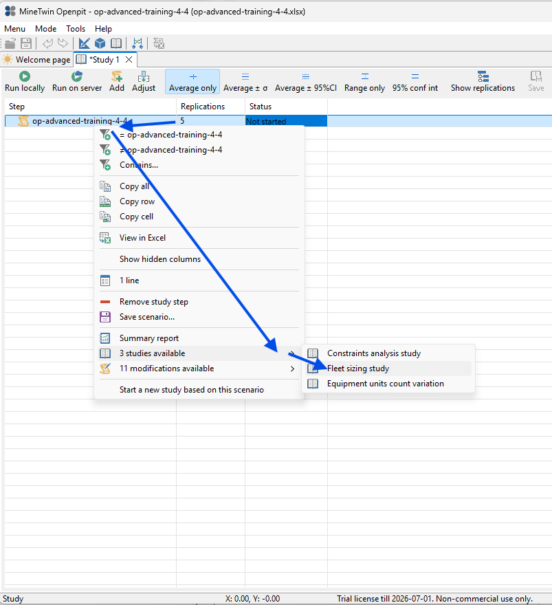
We start a Fleet sizing study from the current scenario and set the number of replications to 5. This allows MineTwin to compare candidate fleet configurations using averaged results across several stochastic runs.

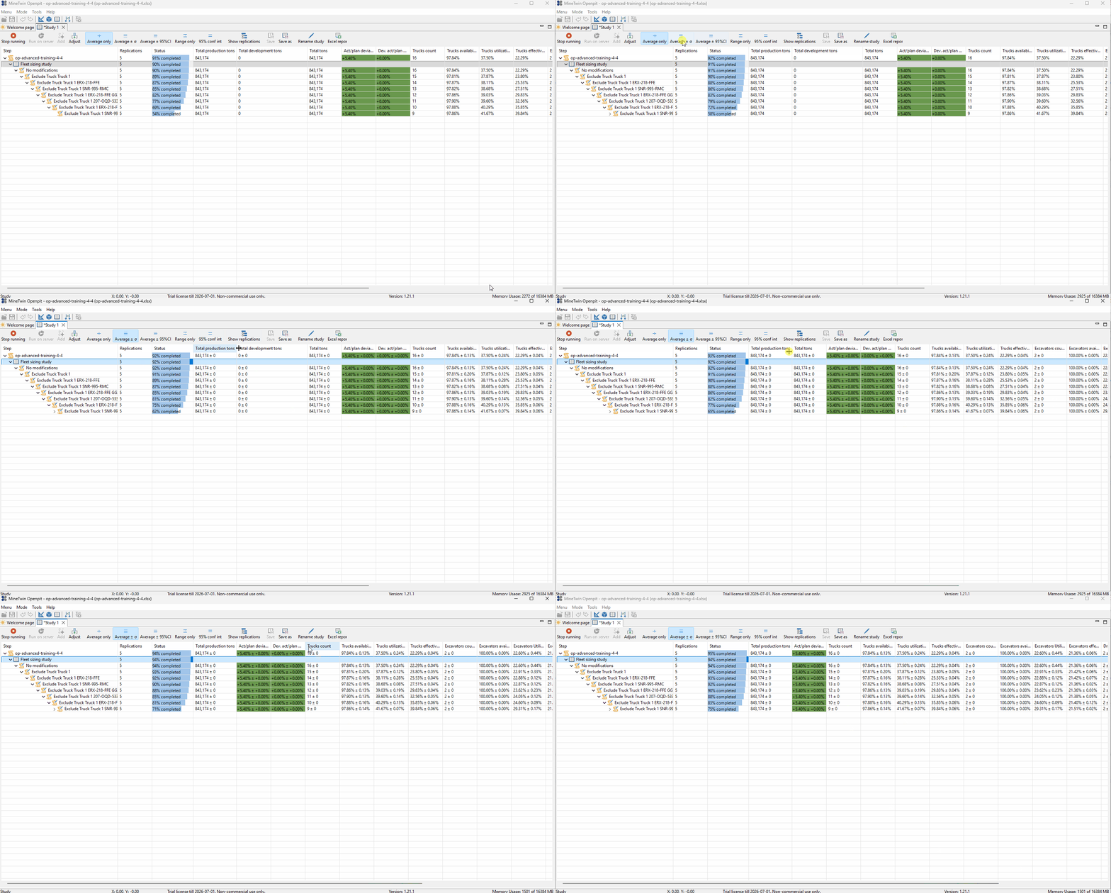
While the study is running, we switch the result view to Average ± σ and adjust the visible columns. This helps us monitor not only the average result, but also the variability of key indicators such as production, availability, utilization, and effective utilization.

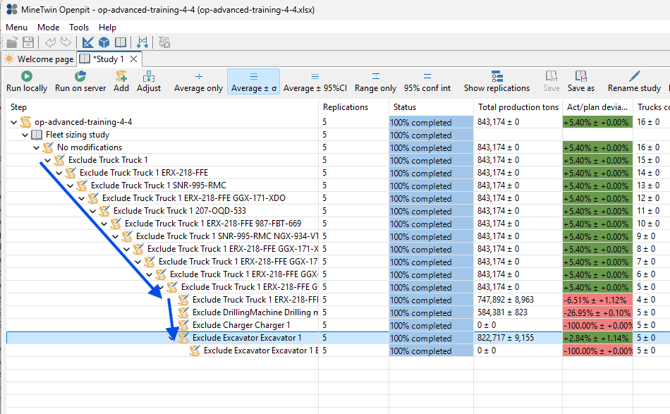
We analyze the completed hierarchical study table. The study removes equipment step by step and checks whether each reduced fleet still reaches the plan. The visible best configuration keeps production above the target with 822,717 t, while reducing the fleet to 5 trucks and 1 excavator.

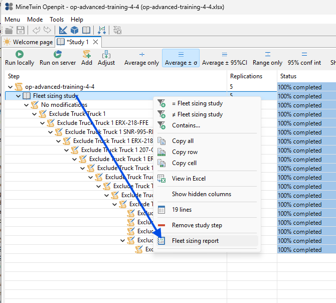
We open the Fleet sizing report from the study context menu. The report summarizes the baseline scenario and the best fleet configuration in a more readable form.

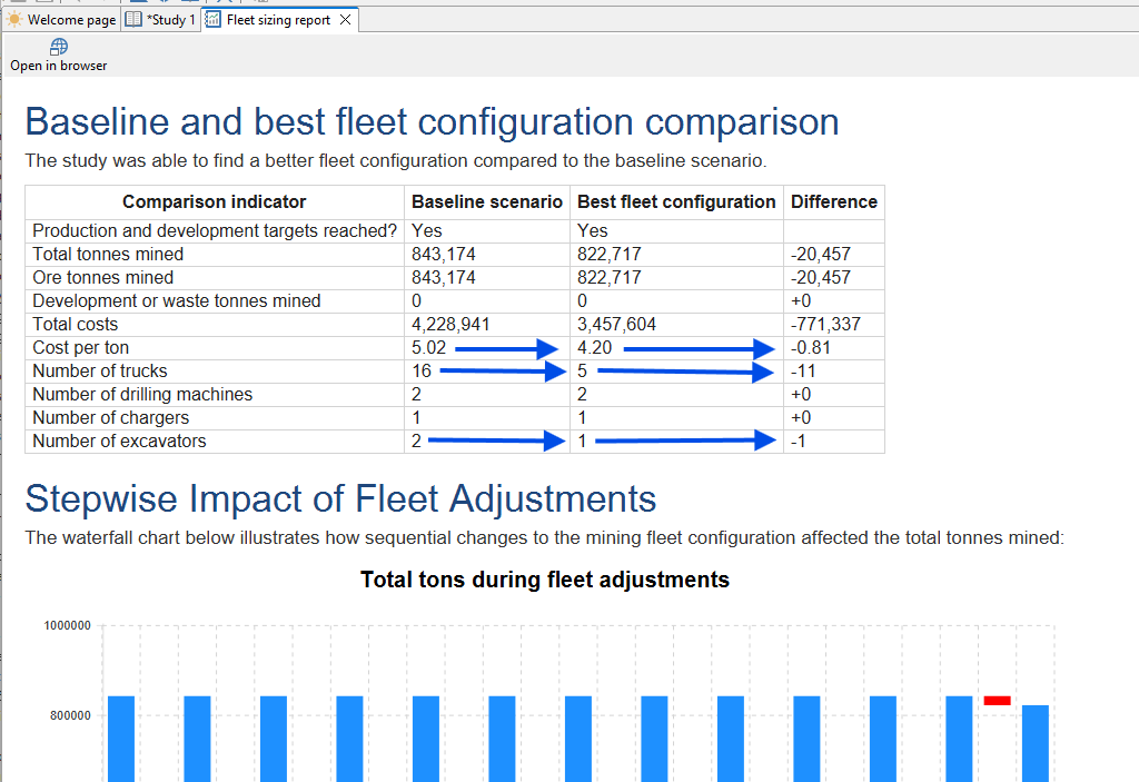
We review the fleet sizing report and compare the baseline with the best fleet configuration. The report shows that both configurations reach the production target, but the best configuration reduces the number of trucks from 16 to 5 and the number of excavators from 2 to 1, while keeping 2 drilling machines and 1 charger. It also reduces cost per ton from 5.02 to 4.20, which shows the economic effect of removing underused equipment.

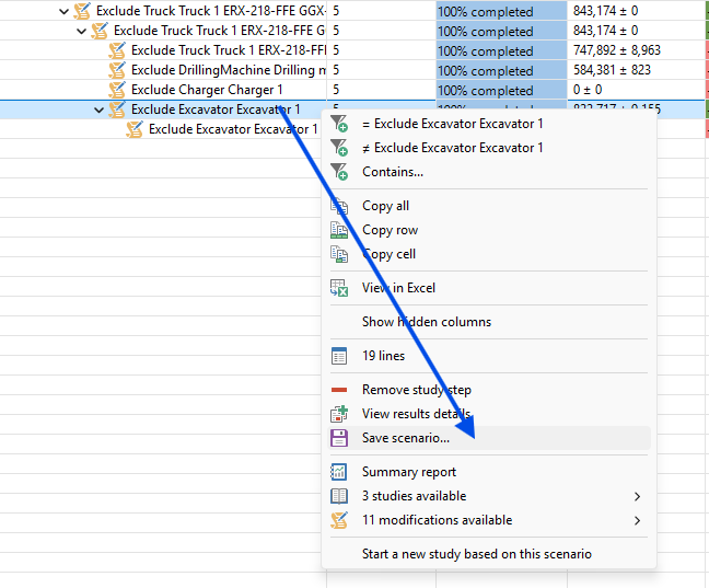
We save the selected best fleet configuration as a separate scenario file. This lets us continue the training from the optimized fleet setup without losing the original study results.

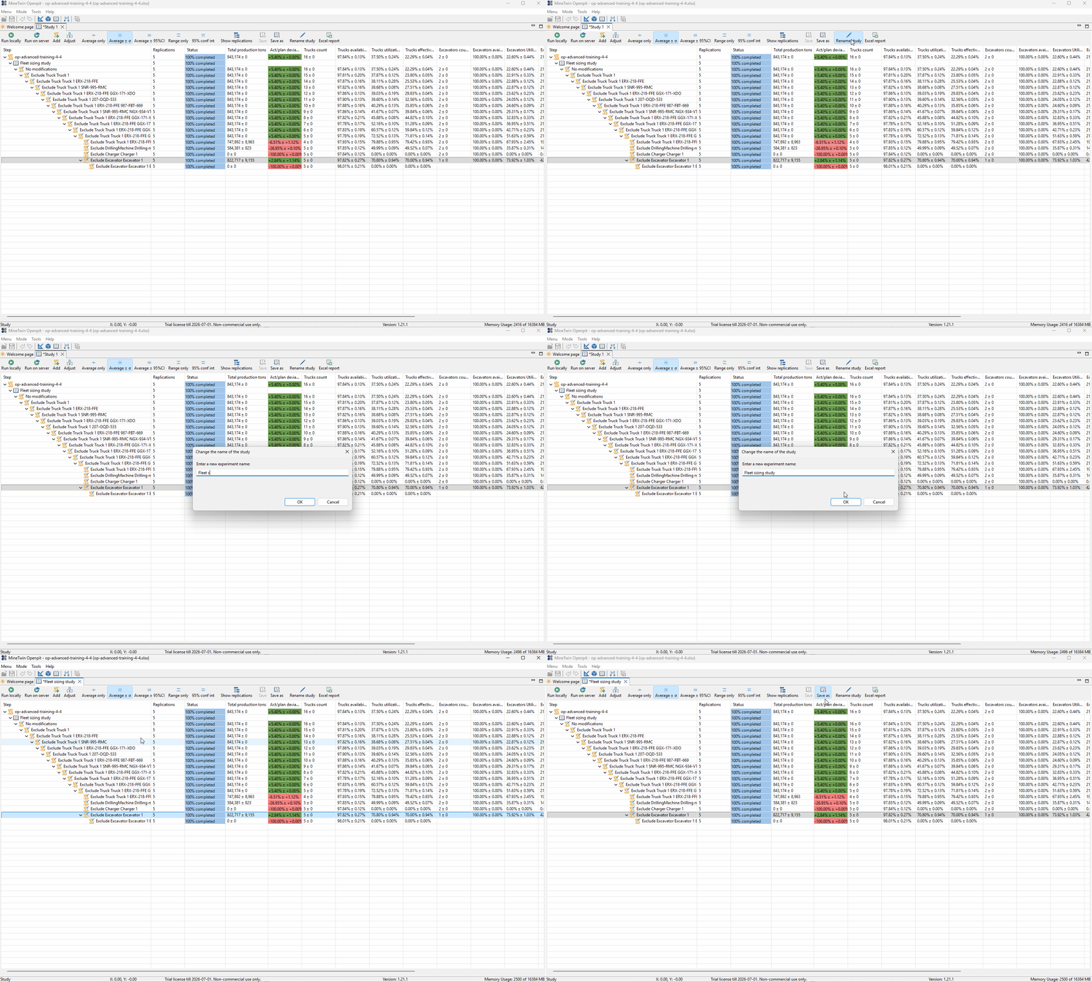
We rename the study and save it to a local study file. This preserves the study tree, all calculated branches, and the report results for later review.

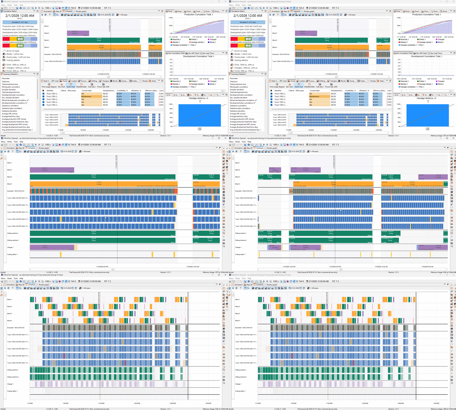
We open the saved scenario and review its simulation Gantt chart. The chart confirms that the reduced fleet still supports the monthly production cycle, with drilling, charging, excavation, haulage, fueling, maintenance, and failure-related interruptions represented in the schedule.

Download scenario

Download study

In this section, we will run a two-parameter sensitivity study. We will vary rolling resistance on the in-pit mine arc and the number of trucks, then compare how these parameters affect production and route speed.

This study helps us understand how robust the fleet configuration is when road conditions change. Because the study contains many simulations, we will run it on the server and use replications to account for stochastic variability.

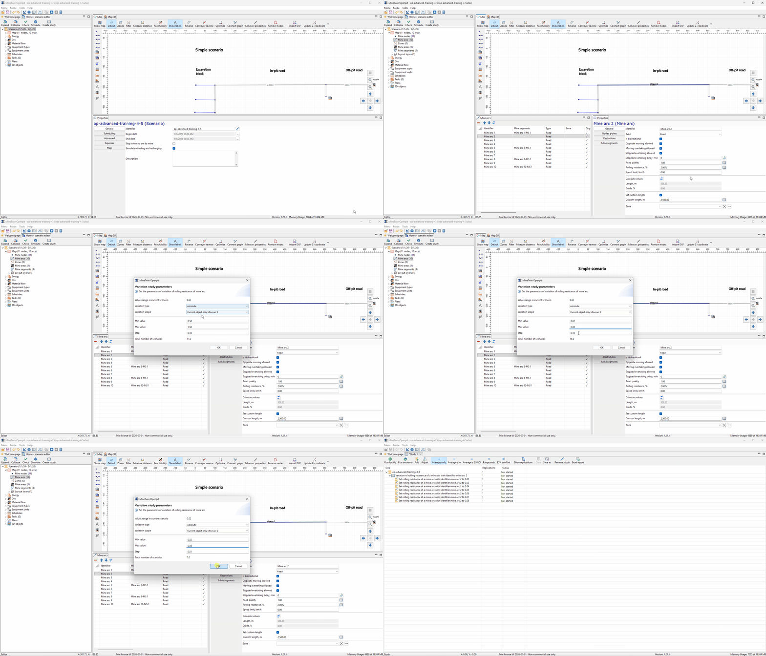
We create a parameter variation study for rolling resistance on mine arc 2. The study tests rolling resistance values from 0.02 to 0.08, so we can represent a range of road conditions for the in-pit haul road.

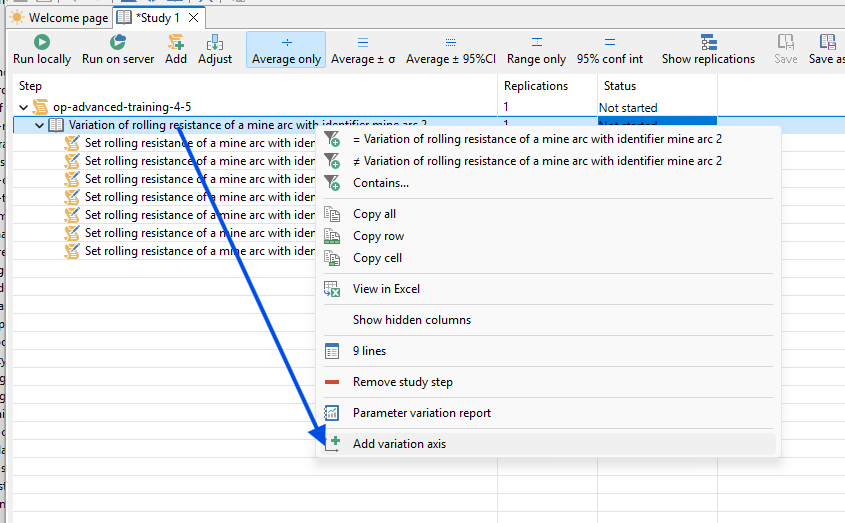
We add a second variation axis to the same study. This turns the study into a two-parameter analysis, where each rolling resistance value will be combined with several truck fleet sizes.

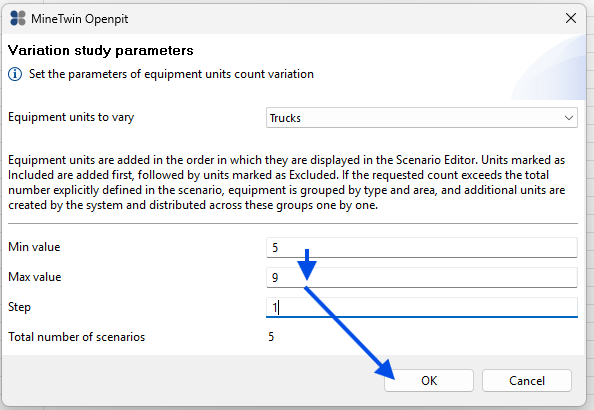
We configure the second axis as a truck count variation. The study will test 5 to 9 trucks with a step of 1, creating five truck count options for each rolling resistance value.

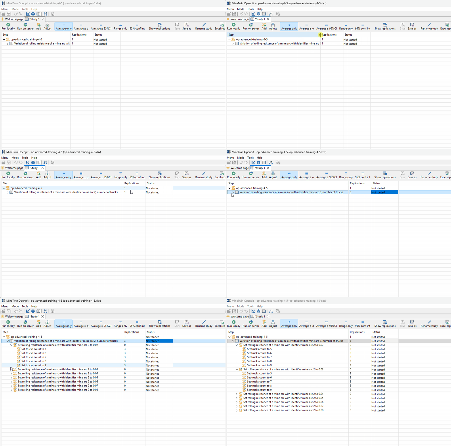
We set 3 replications at the study level. This immediately updates the replication count for every scenario included in the study, so each parameter combination will be calculated three times. As a result, MineTwin will run 105 simulations: 35 parameter combinations with 3 replications each.

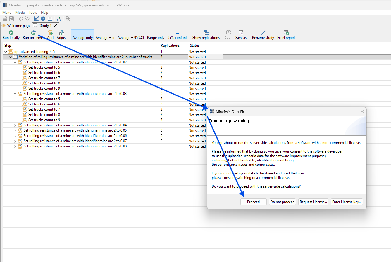
We start the study on the MineTwin execution server and proceed through the data usage warning. Running the study on the server lets the large batch of simulations be calculated outside the desktop application.

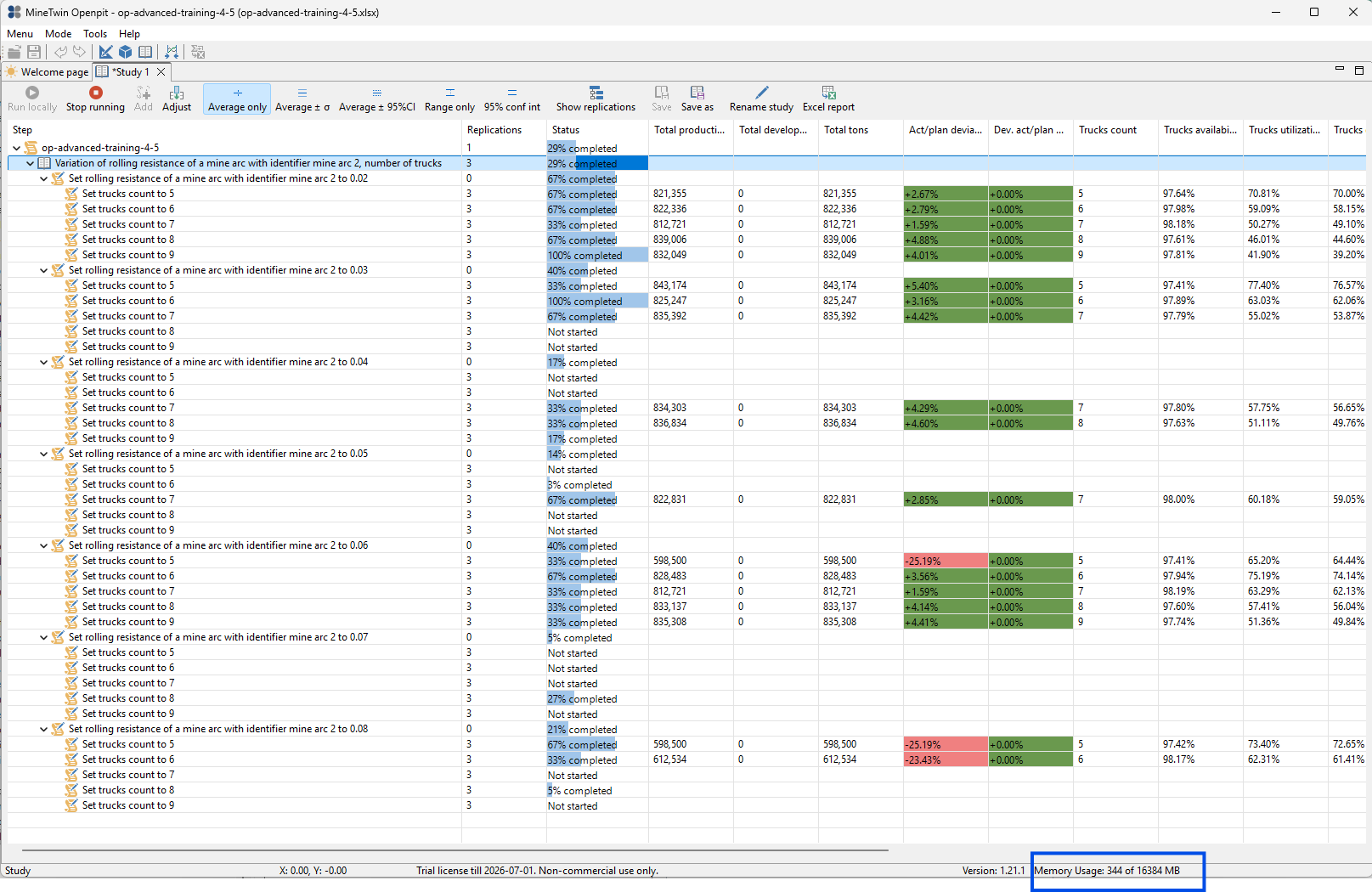
We monitor the study progress while server-side calculations are running. The table shows that multiple branches are being calculated, while the local application uses only a small amount of memory because the simulations are executed on the server.

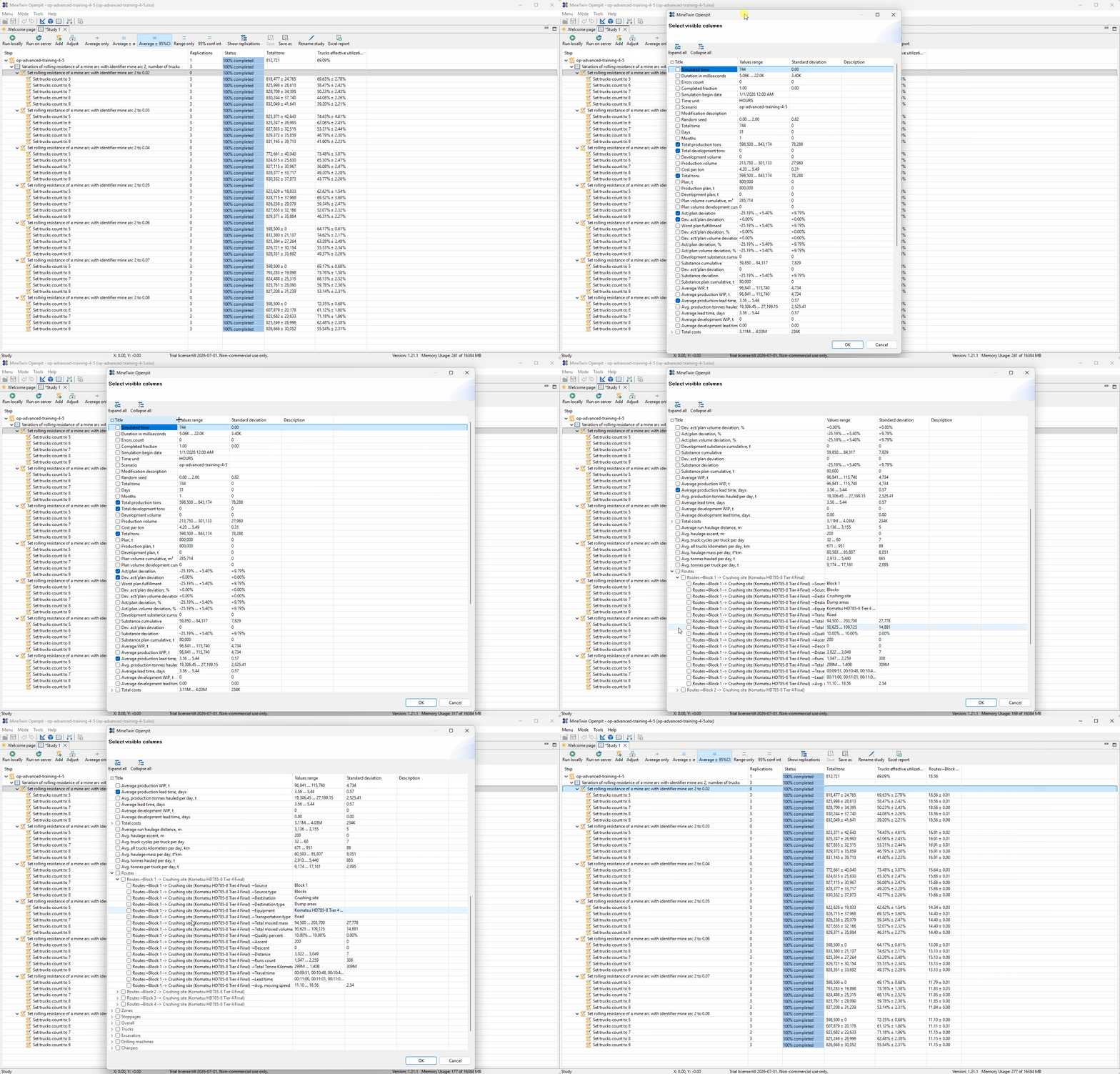
We add the average movement speed indicator for the route from the blocks to the dump area. The result shows that average route speed decreases as rolling resistance increases, which confirms the operational effect of worse road conditions.

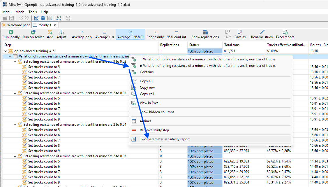
We open the Two-parameter sensitivity report from the study context menu. The report summarizes the calculated grid of rolling resistance and truck count values.

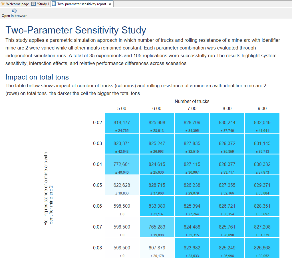
We review the heatmap in the Two-parameter sensitivity report. Rows represent rolling resistance values, columns represent truck counts, and each cell shows the total tons with variability across replications. The report makes it easier to see where additional trucks compensate for higher rolling resistance and where the production target becomes difficult to maintain.

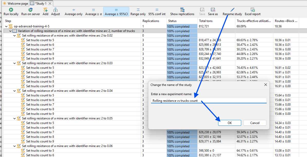
We rename the study to Rolling resistance vs trucks count. This makes the saved study easier to identify later.

Save the study to a local file.

Download scenario

Download study